| Step | Derivation/Formula | Reasoning |
|---|---|---|
| 1 | \( p_{x} = m_{1} v_{i} = 1000 \;\text{kg}\times20\;\text{m/s} = 20000 \;\text{kg}\cdot\text{m/s} \) | This is the momentum in the east (\(x\)) direction for the first car. |
| 2 | \( p_{y} = m_{2} v_{i} = 2000 \;\text{kg}\times15\;\text{m/s} = 30000 \;\text{kg}\cdot\text{m/s} \) | This is the momentum in the north (\(y\)) direction for the second car. |
| 3 | \( p = \sqrt{p_{x}^{2}+p_{y}^{2}} = \sqrt{20000^{2}+30000^{2}} = \sqrt{400\times10^{6}+900\times10^{6}} = \sqrt{1300\times10^{6}} \) | This computes the magnitude of the total momentum after the collision. |
| 4 | \( m_{\text{total}} = m_{1} + m_{2} = 1000 \;\text{kg} + 2000 \;\text{kg} = 3000 \;\text{kg} \) | This is the combined mass of the two cars after the collision. |
| 5 | \( v_{i} = \frac{p}{m_{\text{total}}} = \frac{\sqrt{1300\times10^{6}}}{3000} = \frac{1000\sqrt{1300}}{3000} = \frac{\sqrt{1300}}{3} \;\text{m/s} \) | This gives the speed immediately after the collision (the initial speed for the skid), where \(v_{i}\) is used consistently. |
| 6 | \( \theta = \tan^{-1}\left(\frac{p_{y}}{p_{x}}\right) = \tan^{-1}\left(\frac{30000}{20000}\right) = \tan^{-1}(1.5) \) | This determines the direction of the combined velocity relative to east. (Numerically, \(\tan^{-1}(1.5)\) is approximately \(56.3^\circ\) north of east.) |
| Step | Derivation/Formula | Reasoning |
|---|---|---|
| 1 | \( a = \mu_{k}g = 0.9\times9.8 = 8.82 \;\text{m/s}^{2} \) | This calculates the deceleration due to kinetic friction acting on the combined cars. |
| 2 | \( \Delta x = \frac{v_{i}^{2}}{2a} = \frac{\left(\frac{\sqrt{1300}}{3}\right)^{2}}{2\times0.9\times9.8} = \frac{\frac{1300}{9}}{17.64} \) | We use the kinematic relation for stopping distance when the final velocity is \(v_{x}=0\); here, \(\Delta x\) is the skid distance. |
| 3 | \( \Delta x = \frac{1300}{9\times17.64} \approx 8.19 \;\text{m} \) | This is the calculated skid distance after substituting the numerical values. |
| 4 | \( \boxed{\Delta x \approx 8.19 \;\text{m} \quad\text{and}\quad \theta \approx 56.3^\circ \;\text{north of east}} \) | This row presents the final answers: the cars skid approximately \(8.19\) meters in a direction approximately \(56.3^\circ\) north of east. |
A Major Upgrade To Phy Is Coming Soon — Stay Tuned
We'll help clarify entire units in one hour or less — guaranteed.
Traveling at a speed of 15.9 m/s, the driver of an automobile suddenly locks the wheels by slamming on the brakes. The coefficient of kinetic friction between the tires and the road is 0.659. What is the speed of the automobile after 1.59 s have elapsed? Ignore the effects of air resistance.
Can an object have a non-zero distance and zero average speed?
A 0.035 kg bullet moving horizontally at 350 m/s embeds itself into an initially stationary 0.55 kg block. Air resistance is negligible.
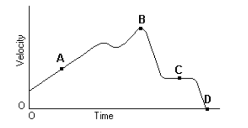 Given the graph of velocity versus time for a duck flying due south for the winter, at what labeled point did the duck stop its forward motion?
A ranger in a national park is driving at \( 56 \, \text{km/h} \) when a deer jumps onto the road \( 65 \, \text{m} \) ahead of the vehicle. After a reaction time of \( t \, \text{s} \), the ranger applies the brakes to produce an acceleration of \( -3 \, \text{m/s}^2 \). What is the maximum reaction time allowed if the ranger is to avoid hitting the deer?
A bowling ball moving with speed \(v\) collides head-on with a stationary tennis ball. The collision is elastic and there is no friction. The bowling ball barely slows down. What is the speed of the tennis ball after the collision?
On a harsh winter day, a \( 1500 \) \( \text{kg} \) vehicle takes a circular banked exit ramp (radius \( R = 150 \) \( \text{m} \); banking angle of \( 10^\circ \)) at a speed of \( 30 \) \( \text{mph} \), since the speed limit is \( 35 \) \( \text{mph} \). However, the exit ramp is completely iced up (frictionless). To make matters worse, a wind is blowing parallel to the ramp in a downward direction. The wind exerts a force of \( 3000 \) \( \text{N} \). Under these conditions, can the driver continue to follow a safe horizontal circle on the exit ramp and stay below the speed limit?
To convert \( \text{mph} \) into \( \text{m/s} \), use \( 1 \) \( \text{mi} = 1607 \) \( \text{m} \) and \( 1 \) \( \text{hr} = 3600 \) \( \text{s} \).
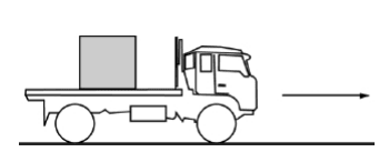
A \( 4700 \, \text{kg} \) truck carrying a \( 900 \, \text{kg} \) crate is traveling at \( 25 \, \text{m/s} \) to the right along a straight, level highway, as shown above. The truck driver then applies the brakes, and as it slows down, the truck travels \( 55 \, \text{m} \) in the next \( 3.0 \, \text{s} \). The crate does not slide on the back of the truck.
A skater glides across the ice at a constant \( 6 \) \( \text{m/s} \). After \( 4 \) \( \text{s} \), friction gradually slows them down until they come to rest in \( 6 \) \( \text{s} \). They pause for \( 2 \) \( \text{s} \), then push off in the opposite direction, steadily gaining speed for \( 5 \) \( \text{s} \). Draw the velocity vs. time graph.
\(\Delta x \approx 8.19 \;\text{m}\) and \(\theta \approx 56.3^\circ\;\text{north of east}\)
By continuing you (1) agree to our Terms of Use and Terms of Sale and (2) consent to sharing your IP and browser information used by this site’s security protocols as outlined in our Privacy Policy.
| Kinematics | Forces |
|---|---|
| \(\Delta x = v_i t + \frac{1}{2} at^2\) | \(F = ma\) |
| \(v = v_i + at\) | \(F_g = \frac{G m_1 m_2}{r^2}\) |
| \(v^2 = v_i^2 + 2a \Delta x\) | \(f = \mu N\) |
| \(\Delta x = \frac{v_i + v}{2} t\) | \(F_s =-kx\) |
| \(v^2 = v_f^2 \,-\, 2a \Delta x\) |
| Circular Motion | Energy |
|---|---|
| \(F_c = \frac{mv^2}{r}\) | \(KE = \frac{1}{2} mv^2\) |
| \(a_c = \frac{v^2}{r}\) | \(PE = mgh\) |
| \(T = 2\pi \sqrt{\frac{r}{g}}\) | \(KE_i + PE_i = KE_f + PE_f\) |
| \(W = Fd \cos\theta\) |
| Momentum | Torque and Rotations |
|---|---|
| \(p = mv\) | \(\tau = r \cdot F \cdot \sin(\theta)\) |
| \(J = \Delta p\) | \(I = \sum mr^2\) |
| \(p_i = p_f\) | \(L = I \cdot \omega\) |
| Simple Harmonic Motion | Fluids |
|---|---|
| \(F = -kx\) | \(P = \frac{F}{A}\) |
| \(T = 2\pi \sqrt{\frac{l}{g}}\) | \(P_{\text{total}} = P_{\text{atm}} + \rho gh\) |
| \(T = 2\pi \sqrt{\frac{m}{k}}\) | \(Q = Av\) |
| \(x(t) = A \cos(\omega t + \phi)\) | \(F_b = \rho V g\) |
| \(a = -\omega^2 x\) | \(A_1v_1 = A_2v_2\) |
| Constant | Description |
|---|---|
| [katex]g[/katex] | Acceleration due to gravity, typically [katex]9.8 , \text{m/s}^2[/katex] on Earth’s surface |
| [katex]G[/katex] | Universal Gravitational Constant, [katex]6.674 \times 10^{-11} , \text{N} \cdot \text{m}^2/\text{kg}^2[/katex] |
| [katex]\mu_k[/katex] and [katex]\mu_s[/katex] | Coefficients of kinetic ([katex]\mu_k[/katex]) and static ([katex]\mu_s[/katex]) friction, dimensionless. Static friction ([katex]\mu_s[/katex]) is usually greater than kinetic friction ([katex]\mu_k[/katex]) as it resists the start of motion. |
| [katex]k[/katex] | Spring constant, in [katex]\text{N/m}[/katex] |
| [katex] M_E = 5.972 \times 10^{24} , \text{kg} [/katex] | Mass of the Earth |
| [katex] M_M = 7.348 \times 10^{22} , \text{kg} [/katex] | Mass of the Moon |
| [katex] M_M = 1.989 \times 10^{30} , \text{kg} [/katex] | Mass of the Sun |
| Variable | SI Unit |
|---|---|
| [katex]s[/katex] (Displacement) | [katex]\text{meters (m)}[/katex] |
| [katex]v[/katex] (Velocity) | [katex]\text{meters per second (m/s)}[/katex] |
| [katex]a[/katex] (Acceleration) | [katex]\text{meters per second squared (m/s}^2\text{)}[/katex] |
| [katex]t[/katex] (Time) | [katex]\text{seconds (s)}[/katex] |
| [katex]m[/katex] (Mass) | [katex]\text{kilograms (kg)}[/katex] |
| Variable | Derived SI Unit |
|---|---|
| [katex]F[/katex] (Force) | [katex]\text{newtons (N)}[/katex] |
| [katex]E[/katex], [katex]PE[/katex], [katex]KE[/katex] (Energy, Potential Energy, Kinetic Energy) | [katex]\text{joules (J)}[/katex] |
| [katex]P[/katex] (Power) | [katex]\text{watts (W)}[/katex] |
| [katex]p[/katex] (Momentum) | [katex]\text{kilogram meters per second (kgm/s)}[/katex] |
| [katex]\omega[/katex] (Angular Velocity) | [katex]\text{radians per second (rad/s)}[/katex] |
| [katex]\tau[/katex] (Torque) | [katex]\text{newton meters (Nm)}[/katex] |
| [katex]I[/katex] (Moment of Inertia) | [katex]\text{kilogram meter squared (kgm}^2\text{)}[/katex] |
| [katex]f[/katex] (Frequency) | [katex]\text{hertz (Hz)}[/katex] |
Metric Prefixes
Example of using unit analysis: Convert 5 kilometers to millimeters.
Start with the given measurement: [katex]\text{5 km}[/katex]
Use the conversion factors for kilometers to meters and meters to millimeters: [katex]\text{5 km} \times \frac{10^3 \, \text{m}}{1 \, \text{km}} \times \frac{10^3 \, \text{mm}}{1 \, \text{m}}[/katex]
Perform the multiplication: [katex]\text{5 km} \times \frac{10^3 \, \text{m}}{1 \, \text{km}} \times \frac{10^3 \, \text{mm}}{1 \, \text{m}} = 5 \times 10^3 \times 10^3 \, \text{mm}[/katex]
Simplify to get the final answer: [katex]\boxed{5 \times 10^6 \, \text{mm}}[/katex]
Prefix | Symbol | Power of Ten | Equivalent |
|---|---|---|---|
Pico- | p | [katex]10^{-12}[/katex] | 0.000000000001 |
Nano- | n | [katex]10^{-9}[/katex] | 0.000000001 |
Micro- | µ | [katex]10^{-6}[/katex] | 0.000001 |
Milli- | m | [katex]10^{-3}[/katex] | 0.001 |
Centi- | c | [katex]10^{-2}[/katex] | 0.01 |
Deci- | d | [katex]10^{-1}[/katex] | 0.1 |
(Base unit) | – | [katex]10^{0}[/katex] | 1 |
Deca- or Deka- | da | [katex]10^{1}[/katex] | 10 |
Hecto- | h | [katex]10^{2}[/katex] | 100 |
Kilo- | k | [katex]10^{3}[/katex] | 1,000 |
Mega- | M | [katex]10^{6}[/katex] | 1,000,000 |
Giga- | G | [katex]10^{9}[/katex] | 1,000,000,000 |
Tera- | T | [katex]10^{12}[/katex] | 1,000,000,000,000 |
One price to unlock most advanced version of Phy across all our tools.
per month
Billed Monthly. Cancel Anytime.
We crafted THE Ultimate A.P Physics 1 Program so you can learn faster and score higher.
Try our free calculator to see what you need to get a 5 on the 2026 AP Physics 1 exam.
A quick explanation
Credits are used to grade your FRQs and GQs. Pro users get unlimited credits.
Submitting counts as 1 attempt.
Viewing answers or explanations count as a failed attempts.
Phy gives partial credit if needed
MCQs and GQs are are 1 point each. FRQs will state points for each part.
Phy customizes problem explanations based on what you struggle with. Just hit the explanation button to see.
Understand you mistakes quicker.

Phy automatically provides feedback so you can improve your responses.
10 Free Credits To Get You Started

By continuing you agree to nerd-notes.com Terms of Service, Privacy Policy, and our usage of user data.
Feeling uneasy about your next physics test? We'll boost your grade in 3 lessons or less—guaranteed

NEW! PHY AI accurately solves all questions
🔥 Get up to 30% off Elite Physics Tutoring
🧠 NEW! Learn Physics From Scratch Self Paced Course
🎯 Need exam style practice questions?
