| Step | Derivation/Formula | Reasoning |
|---|---|---|
| 1 | \(\frac{d}{dt}(v(t)) = a(t) = 18t\) | Given the acceleration function \(a(t) = 18t\), integrate to find the velocity function. |
| 2 | \(v(t) = \int 18t \, dt\) | Integrate the acceleration to find the velocity. This involves indefinite integration of the function \(18t\). |
| 3 | \(v(t) = 9t^2 + C\) | Upon integration, calculate the velocity function. Here \(C\) is the integration constant. |
| 4 | \(v(0) = -12\) | Use the initial condition to find the value of \(C\). At \(t=0\), the velocity \(v(0) = -12 \, \text{m/s}\). |
| 5 | \(-12 = 9(0)^2 + C \Rightarrow C = -12\) | Substitute the initial condition into the velocity function to solve for \(C\). |
| 6 | \(v(t) = 9t^2 – 12\) | Substitute the value of \(C\) back into the velocity function. |
| 7 | \(x(t) = \int v(t) \, dt\) | Integrate the velocity function to find the position function. |
| 8 | \(x(t) = \int (9t^2 – 12) \, dt\) | Set up the indefinite integral of the velocity function. |
| 9 | \(x(t) = 3t^3 – 12t + C’\) | Integrate to find the position function, where \(C’\) is another integration constant. |
| 10 | \(x(0) = 0\) | Use the initial condition to find the value of \(C’\). At \(t=0\), the position \(x(0) = 0 \, \text{m}\). |
| 11 | \(0 = 3(0)^3 – 12(0) + C’ \Rightarrow C’ = 0\) | Substitute the initial condition into the position function to solve for \(C’\). |
| 12 | \(x(t) = 3t^3 – 12t\) | Substitute the value of \(C’\) back into the position function. Now the position function is completely determined. |
| 13 | \(x(4) = 3(4)^3 – 12(4) = 3(64) – 48 = 192 – 48 = 144\) | Evaluate the position function at \(t = 4.0 \, \text{s}\). |
| 14 | \(x = 144 \, \text{m}\) | The position of the particle at \(t = 4.0 \, \text{s}\) is \(\boxed{144 \, \text{m}}\). |
The correct answer is (d) 144 m.
A Major Upgrade To Phy Is Coming Soon — Stay Tuned
We'll help clarify entire units in one hour or less — guaranteed.
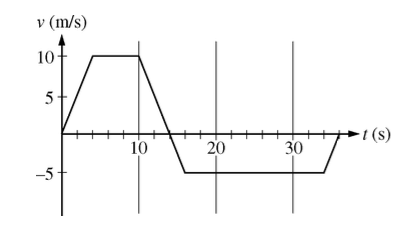
Above is the graph of an object’s velocity as a function of time. Which of the following is true about the motion?
What does displacement mean in the context of motion?
A horizontal spring with spring constant 162 N/m is compressed 50 cm and used to launch a 3 kg box across a frictionless, horizontal surface. After the box travels some distance, the surface becomes rough. The coefficient of kinetic friction of the box on the rough surface is 0.2. Find the total distance the box travels before stopping.
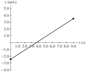
The motion of a particle is described in the velocity vs. time graph shown above. Over the nine-second interval shown, we can say that the speed of the particle…
A baseball is thrown vertically into the air with a velocity \( v \), and reaches a maximum height \( h \). At what height was the baseball moving with one-half its original velocity? Assume air resistance is negligible.
An object is projected vertically upward from ground level. It rises to a maximum height [katex] H [/katex]. If air resistance is negligible, which of the following must be true for the object when it is at a height [katex] H/2 [/katex] ?
A ball is tossed directly upward. Its total time in the air is \( T \). Its maximum height is \( H \). What is its height after it has been in the air a time \( T/4 \)? Air resistance is negligible.
You drive \( 4 \) \( \text{km} \) at \( 30 \) \( \text{km/h} \) and then another \( 4 \) \( \text{km} \) at \( 50 \) \( \text{km/h} \). What is your average speed for the whole \( 8 \) \( \text{km} \) trip?
An object undergoes constant acceleration. Starting from rest, the object travels \( 5 \, \text{m} \) in the first second. Then it travels \( 15 \, \text{m} \) in the next second. What total distance will be covered after the 3rd second?
A car is heading rightward but accelerating to the left. This means the car is:
By continuing you (1) agree to our Terms of Use and Terms of Sale and (2) consent to sharing your IP and browser information used by this site’s security protocols as outlined in our Privacy Policy.
| Kinematics | Forces |
|---|---|
| \(\Delta x = v_i t + \frac{1}{2} at^2\) | \(F = ma\) |
| \(v = v_i + at\) | \(F_g = \frac{G m_1 m_2}{r^2}\) |
| \(v^2 = v_i^2 + 2a \Delta x\) | \(f = \mu N\) |
| \(\Delta x = \frac{v_i + v}{2} t\) | \(F_s =-kx\) |
| \(v^2 = v_f^2 \,-\, 2a \Delta x\) |
| Circular Motion | Energy |
|---|---|
| \(F_c = \frac{mv^2}{r}\) | \(KE = \frac{1}{2} mv^2\) |
| \(a_c = \frac{v^2}{r}\) | \(PE = mgh\) |
| \(T = 2\pi \sqrt{\frac{r}{g}}\) | \(KE_i + PE_i = KE_f + PE_f\) |
| \(W = Fd \cos\theta\) |
| Momentum | Torque and Rotations |
|---|---|
| \(p = mv\) | \(\tau = r \cdot F \cdot \sin(\theta)\) |
| \(J = \Delta p\) | \(I = \sum mr^2\) |
| \(p_i = p_f\) | \(L = I \cdot \omega\) |
| Simple Harmonic Motion | Fluids |
|---|---|
| \(F = -kx\) | \(P = \frac{F}{A}\) |
| \(T = 2\pi \sqrt{\frac{l}{g}}\) | \(P_{\text{total}} = P_{\text{atm}} + \rho gh\) |
| \(T = 2\pi \sqrt{\frac{m}{k}}\) | \(Q = Av\) |
| \(x(t) = A \cos(\omega t + \phi)\) | \(F_b = \rho V g\) |
| \(a = -\omega^2 x\) | \(A_1v_1 = A_2v_2\) |
| Constant | Description |
|---|---|
| [katex]g[/katex] | Acceleration due to gravity, typically [katex]9.8 , \text{m/s}^2[/katex] on Earth’s surface |
| [katex]G[/katex] | Universal Gravitational Constant, [katex]6.674 \times 10^{-11} , \text{N} \cdot \text{m}^2/\text{kg}^2[/katex] |
| [katex]\mu_k[/katex] and [katex]\mu_s[/katex] | Coefficients of kinetic ([katex]\mu_k[/katex]) and static ([katex]\mu_s[/katex]) friction, dimensionless. Static friction ([katex]\mu_s[/katex]) is usually greater than kinetic friction ([katex]\mu_k[/katex]) as it resists the start of motion. |
| [katex]k[/katex] | Spring constant, in [katex]\text{N/m}[/katex] |
| [katex] M_E = 5.972 \times 10^{24} , \text{kg} [/katex] | Mass of the Earth |
| [katex] M_M = 7.348 \times 10^{22} , \text{kg} [/katex] | Mass of the Moon |
| [katex] M_M = 1.989 \times 10^{30} , \text{kg} [/katex] | Mass of the Sun |
| Variable | SI Unit |
|---|---|
| [katex]s[/katex] (Displacement) | [katex]\text{meters (m)}[/katex] |
| [katex]v[/katex] (Velocity) | [katex]\text{meters per second (m/s)}[/katex] |
| [katex]a[/katex] (Acceleration) | [katex]\text{meters per second squared (m/s}^2\text{)}[/katex] |
| [katex]t[/katex] (Time) | [katex]\text{seconds (s)}[/katex] |
| [katex]m[/katex] (Mass) | [katex]\text{kilograms (kg)}[/katex] |
| Variable | Derived SI Unit |
|---|---|
| [katex]F[/katex] (Force) | [katex]\text{newtons (N)}[/katex] |
| [katex]E[/katex], [katex]PE[/katex], [katex]KE[/katex] (Energy, Potential Energy, Kinetic Energy) | [katex]\text{joules (J)}[/katex] |
| [katex]P[/katex] (Power) | [katex]\text{watts (W)}[/katex] |
| [katex]p[/katex] (Momentum) | [katex]\text{kilogram meters per second (kgm/s)}[/katex] |
| [katex]\omega[/katex] (Angular Velocity) | [katex]\text{radians per second (rad/s)}[/katex] |
| [katex]\tau[/katex] (Torque) | [katex]\text{newton meters (Nm)}[/katex] |
| [katex]I[/katex] (Moment of Inertia) | [katex]\text{kilogram meter squared (kgm}^2\text{)}[/katex] |
| [katex]f[/katex] (Frequency) | [katex]\text{hertz (Hz)}[/katex] |
Metric Prefixes
Example of using unit analysis: Convert 5 kilometers to millimeters.
Start with the given measurement: [katex]\text{5 km}[/katex]
Use the conversion factors for kilometers to meters and meters to millimeters: [katex]\text{5 km} \times \frac{10^3 \, \text{m}}{1 \, \text{km}} \times \frac{10^3 \, \text{mm}}{1 \, \text{m}}[/katex]
Perform the multiplication: [katex]\text{5 km} \times \frac{10^3 \, \text{m}}{1 \, \text{km}} \times \frac{10^3 \, \text{mm}}{1 \, \text{m}} = 5 \times 10^3 \times 10^3 \, \text{mm}[/katex]
Simplify to get the final answer: [katex]\boxed{5 \times 10^6 \, \text{mm}}[/katex]
Prefix | Symbol | Power of Ten | Equivalent |
|---|---|---|---|
Pico- | p | [katex]10^{-12}[/katex] | 0.000000000001 |
Nano- | n | [katex]10^{-9}[/katex] | 0.000000001 |
Micro- | µ | [katex]10^{-6}[/katex] | 0.000001 |
Milli- | m | [katex]10^{-3}[/katex] | 0.001 |
Centi- | c | [katex]10^{-2}[/katex] | 0.01 |
Deci- | d | [katex]10^{-1}[/katex] | 0.1 |
(Base unit) | – | [katex]10^{0}[/katex] | 1 |
Deca- or Deka- | da | [katex]10^{1}[/katex] | 10 |
Hecto- | h | [katex]10^{2}[/katex] | 100 |
Kilo- | k | [katex]10^{3}[/katex] | 1,000 |
Mega- | M | [katex]10^{6}[/katex] | 1,000,000 |
Giga- | G | [katex]10^{9}[/katex] | 1,000,000,000 |
Tera- | T | [katex]10^{12}[/katex] | 1,000,000,000,000 |
One price to unlock most advanced version of Phy across all our tools.
per month
Billed Monthly. Cancel Anytime.
We crafted THE Ultimate A.P Physics 1 Program so you can learn faster and score higher.
Try our free calculator to see what you need to get a 5 on the 2026 AP Physics 1 exam.
A quick explanation
Credits are used to grade your FRQs and GQs. Pro users get unlimited credits.
Submitting counts as 1 attempt.
Viewing answers or explanations count as a failed attempts.
Phy gives partial credit if needed
MCQs and GQs are are 1 point each. FRQs will state points for each part.
Phy customizes problem explanations based on what you struggle with. Just hit the explanation button to see.
Understand you mistakes quicker.

Phy automatically provides feedback so you can improve your responses.
10 Free Credits To Get You Started

By continuing you agree to nerd-notes.com Terms of Service, Privacy Policy, and our usage of user data.
Feeling uneasy about your next physics test? We'll boost your grade in 3 lessons or less—guaranteed

NEW! PHY AI accurately solves all questions
🔥 Get up to 30% off Elite Physics Tutoring
🧠 NEW! Learn Physics From Scratch Self Paced Course
🎯 Need exam style practice questions?
