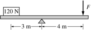
An object weighing 120 N is set on a rigid beam of negligible mass at a distance of 3 m from a pivot, as shown above. A vertical force is to be applied to the other end of the beam a distance of 4 m from the pivot to keep the beam at rest and horizontal. What is the magnitude F of the force required?
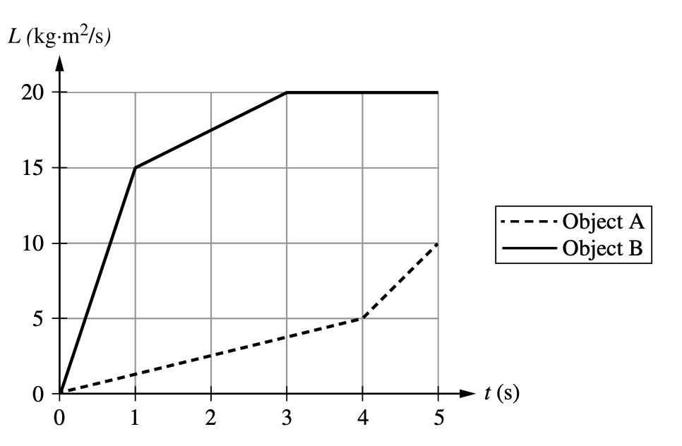
Two disks, A and B, each experience a net external torque that varies over an interval of \( 5 \) \( \text{s} \). Disk B has a rotational inertia that is twice that of Disk A. The graph shown represents the angular momentum of the two disks as functions of time between \( t = 0 \) \( \text{s} \) and \( t = 5 \) \( \text{s} \). The average magnitudes of the net torques exerted on disks A and B from \( t = 0 \) \( \text{s} \) to \( t = 5 \) \( \text{s} \) are \( \tau_A \) and \( \tau_B \), respectively. Which of the following expressions correctly relates the magnitudes of the average torques?
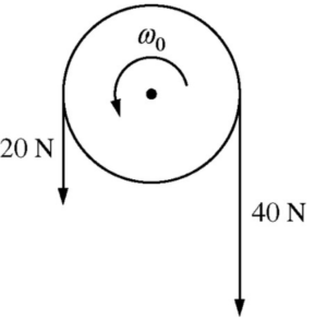
A disk is initially rotating counterclockwise around a fixed axis with angular speed \( \omega_0 \). At time \( t = 0 \), the two forces shown in the figure above are exerted on the disk. If counterclockwise is positive, which of the following could show the angular velocity of the disk as a function of time?


