| Step | Derivation/Formula | Reasoning |
|---|---|---|
| 1 | \[\rho = R – r\] | Because the ball rolls on the inside of the track, its center is offset inward by its radius. Thus, the center follows a circular path of radius \(\rho = R – r\). |
| 2 | \[\Delta h = R – r\] | At the vertical edge the ball’s center is at a height of \(0\) (relative to the track center chosen so that the lowest point is \(- (R – r)\)) and at the lowest point it is at \(y = -(R – r)\); hence the drop in height is \(R – r\). |
| 3 | \[m g (R – r) = \frac{1}{2} m v_x^2 + \frac{1}{2} I \omega^2\] | Applying conservation of energy: the loss in gravitational potential energy equals the sum of translational and rotational kinetic energies. |
| 4 | \[I = \frac{2}{5} m r^2 \quad \text{and} \quad v_x = \omega r\] | For a solid spherical ball, the moment of inertia is \(\frac{2}{5} m r^2\) and rolling without slipping implies \(v_x = \omega r\). |
| 5 | \[\frac{1}{2} m v_x^2 + \frac{1}{2}\left(\frac{2}{5}m r^2\right)\left(\frac{v_x}{r}\right)^2 = \frac{1}{2} m v_x^2 + \frac{1}{5} m v_x^2 = \frac{7}{10}m v_x^2\] | Substitute the moment of inertia and the no-slip condition to express the rotational kinetic energy in terms of \(v_x\), then combine both kinetic energies. |
| 6 | \[m g (R – r) = \frac{7}{10} m v_x^2\] | Set the gravitational potential energy lost equal to the total kinetic energy gained. |
| 7 | \[v_x^2 = \frac{10}{7} g (R – r)\] | Simplify by canceling \(m\) and solving for \(v_x^2\). |
| 8 | \[\boxed{v_x = \sqrt{\frac{10}{7} g (R – r)}}\] | Take the square root to obtain the final expression for the ball’s speed at the lowest point. |
A Major Upgrade To Phy Is Coming Soon — Stay Tuned

We'll help clarify entire units in one hour or less — guaranteed.
A self paced course with videos, problems sets, and everything you need to get a 5. Trusted by over 15k students and over 200 schools.
Two forces produce equal torques on a door about the door hinge. The first force is applied at the midpoint of the door; the second force is applied at the doorknob. Both forces are applied perpendicular to the door. Which force has a greater magnitude?
A linear spring of negligible mass requires a force of \( 18.0 \, \text{N} \) to cause its length to increase by \( 1.0 \, \text{cm} \). A sphere of mass \( 75.0 \, \text{g} \) is then attached to one end of the spring. The distance between the center of the sphere \( M \) and the other end \( P \) of the un-stretched spring is \( 25.0 \, \text{cm} \). Then the sphere begins rotating at constant speed in a horizontal circle around the center \( P \). The distance \( P \) and \( M \) increases to \( 26.5 \, \text{cm} \).
A rotating merry-go-round makes one complete revolution in 4.0 s. What is the linear speed and acceleration of a child seated 1.2 m from the center?
A sphere of mass \( M \) and radius \( r \), and rotational inertia \( I \) is released from the top of an inclined plane of height \( h \). The surface has considerable friction. Using only the variables mentioned, derive an expression for the sphere’s center of mass velocity.
Ball \(A\) of mass \(m\) is dropped from a building of height \(H\). Ball \(B\) of mass \(1.7 \, \text{m}\) is dropped from a building of height \(1.7H\). Using energy, what the ratio of \(v_A\) to \(v_B\) (final velocity of ball \(A\) to final velocity of ball \(B\)). Air resistance is negligible.
A \(25 \, \text{g}\) steel ball is attached to the top of a \(24 \, \text{cm}\)-diameter vertical wheel of negligible mass. Starting from rest, the wheel accelerates at \(470 \, \text{rad/s}^2\). The ball is released after \(\frac{3}{4}\) of a revolution. How high does it go above the center of the wheel?
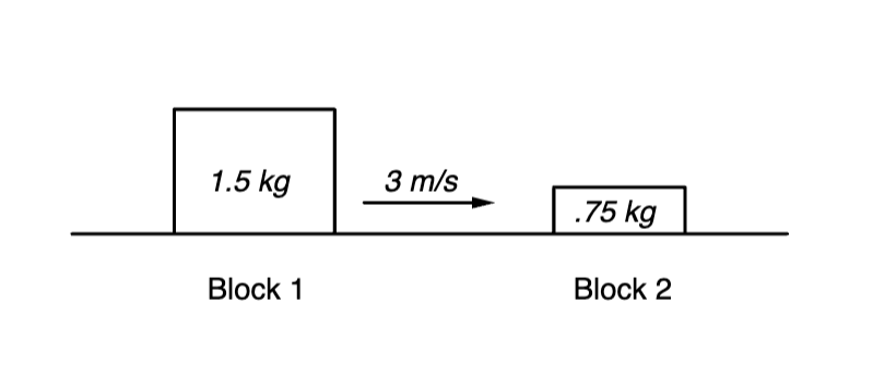
Block 2 initially is at rest. Block 1 travels towards block 2 and collides with Block 2 as shown above. Find the final velocities of both blocks assuming the collision is elastic.
Suppose a solid uniform sphere of mass M and radius R rolls without slipping down an inclined plane starting from rest. The angular velocity of the sphere at the bottom of the incline depends on
A \(6 \, \text{kg}\) cube rests against a compressed spring with a force constant of \(1{,}800 \, \text{N/m}\), initially compressed by \(0.3 \, \text{m}\). Upon release, the cube slides on a horizontal surface with a kinetic friction coefficient of \(\mu_k = 0.12\) for \(3 \, \text{m}\), then ascends a \(12^\circ\) slope, stopping after \(4.5 \, \text{m}\). Determine the coefficient of kinetic friction on the slope.
A friend is balancing a fork on one finger. Which of the following are correct explanations of how he accomplishes this? Select two answers.
\(\boxed{v_x = \sqrt{\frac{10}{7} g (R – r)}}\)
By continuing you (1) agree to our Terms of Use and Terms of Sale and (2) consent to sharing your IP and browser information used by this site’s security protocols as outlined in our Privacy Policy.
| Kinematics | Forces |
|---|---|
| \(\Delta x = v_i t + \frac{1}{2} at^2\) | \(F = ma\) |
| \(v = v_i + at\) | \(F_g = \frac{G m_1 m_2}{r^2}\) |
| \(v^2 = v_i^2 + 2a \Delta x\) | \(f = \mu N\) |
| \(\Delta x = \frac{v_i + v}{2} t\) | \(F_s =-kx\) |
| \(v^2 = v_f^2 \,-\, 2a \Delta x\) |
| Circular Motion | Energy |
|---|---|
| \(F_c = \frac{mv^2}{r}\) | \(KE = \frac{1}{2} mv^2\) |
| \(a_c = \frac{v^2}{r}\) | \(PE = mgh\) |
| \(T = 2\pi \sqrt{\frac{r}{g}}\) | \(KE_i + PE_i = KE_f + PE_f\) |
| \(W = Fd \cos\theta\) |
| Momentum | Torque and Rotations |
|---|---|
| \(p = mv\) | \(\tau = r \cdot F \cdot \sin(\theta)\) |
| \(J = \Delta p\) | \(I = \sum mr^2\) |
| \(p_i = p_f\) | \(L = I \cdot \omega\) |
| Simple Harmonic Motion | Fluids |
|---|---|
| \(F = -kx\) | \(P = \frac{F}{A}\) |
| \(T = 2\pi \sqrt{\frac{l}{g}}\) | \(P_{\text{total}} = P_{\text{atm}} + \rho gh\) |
| \(T = 2\pi \sqrt{\frac{m}{k}}\) | \(Q = Av\) |
| \(x(t) = A \cos(\omega t + \phi)\) | \(F_b = \rho V g\) |
| \(a = -\omega^2 x\) | \(A_1v_1 = A_2v_2\) |
| Constant | Description |
|---|---|
| [katex]g[/katex] | Acceleration due to gravity, typically [katex]9.8 , \text{m/s}^2[/katex] on Earth’s surface |
| [katex]G[/katex] | Universal Gravitational Constant, [katex]6.674 \times 10^{-11} , \text{N} \cdot \text{m}^2/\text{kg}^2[/katex] |
| [katex]\mu_k[/katex] and [katex]\mu_s[/katex] | Coefficients of kinetic ([katex]\mu_k[/katex]) and static ([katex]\mu_s[/katex]) friction, dimensionless. Static friction ([katex]\mu_s[/katex]) is usually greater than kinetic friction ([katex]\mu_k[/katex]) as it resists the start of motion. |
| [katex]k[/katex] | Spring constant, in [katex]\text{N/m}[/katex] |
| [katex] M_E = 5.972 \times 10^{24} , \text{kg} [/katex] | Mass of the Earth |
| [katex] M_M = 7.348 \times 10^{22} , \text{kg} [/katex] | Mass of the Moon |
| [katex] M_M = 1.989 \times 10^{30} , \text{kg} [/katex] | Mass of the Sun |
| Variable | SI Unit |
|---|---|
| [katex]s[/katex] (Displacement) | [katex]\text{meters (m)}[/katex] |
| [katex]v[/katex] (Velocity) | [katex]\text{meters per second (m/s)}[/katex] |
| [katex]a[/katex] (Acceleration) | [katex]\text{meters per second squared (m/s}^2\text{)}[/katex] |
| [katex]t[/katex] (Time) | [katex]\text{seconds (s)}[/katex] |
| [katex]m[/katex] (Mass) | [katex]\text{kilograms (kg)}[/katex] |
| Variable | Derived SI Unit |
|---|---|
| [katex]F[/katex] (Force) | [katex]\text{newtons (N)}[/katex] |
| [katex]E[/katex], [katex]PE[/katex], [katex]KE[/katex] (Energy, Potential Energy, Kinetic Energy) | [katex]\text{joules (J)}[/katex] |
| [katex]P[/katex] (Power) | [katex]\text{watts (W)}[/katex] |
| [katex]p[/katex] (Momentum) | [katex]\text{kilogram meters per second (kgm/s)}[/katex] |
| [katex]\omega[/katex] (Angular Velocity) | [katex]\text{radians per second (rad/s)}[/katex] |
| [katex]\tau[/katex] (Torque) | [katex]\text{newton meters (Nm)}[/katex] |
| [katex]I[/katex] (Moment of Inertia) | [katex]\text{kilogram meter squared (kgm}^2\text{)}[/katex] |
| [katex]f[/katex] (Frequency) | [katex]\text{hertz (Hz)}[/katex] |
Metric Prefixes
Example of using unit analysis: Convert 5 kilometers to millimeters.
Start with the given measurement: [katex]\text{5 km}[/katex]
Use the conversion factors for kilometers to meters and meters to millimeters: [katex]\text{5 km} \times \frac{10^3 \, \text{m}}{1 \, \text{km}} \times \frac{10^3 \, \text{mm}}{1 \, \text{m}}[/katex]
Perform the multiplication: [katex]\text{5 km} \times \frac{10^3 \, \text{m}}{1 \, \text{km}} \times \frac{10^3 \, \text{mm}}{1 \, \text{m}} = 5 \times 10^3 \times 10^3 \, \text{mm}[/katex]
Simplify to get the final answer: [katex]\boxed{5 \times 10^6 \, \text{mm}}[/katex]
Prefix | Symbol | Power of Ten | Equivalent |
|---|---|---|---|
Pico- | p | [katex]10^{-12}[/katex] | 0.000000000001 |
Nano- | n | [katex]10^{-9}[/katex] | 0.000000001 |
Micro- | µ | [katex]10^{-6}[/katex] | 0.000001 |
Milli- | m | [katex]10^{-3}[/katex] | 0.001 |
Centi- | c | [katex]10^{-2}[/katex] | 0.01 |
Deci- | d | [katex]10^{-1}[/katex] | 0.1 |
(Base unit) | – | [katex]10^{0}[/katex] | 1 |
Deca- or Deka- | da | [katex]10^{1}[/katex] | 10 |
Hecto- | h | [katex]10^{2}[/katex] | 100 |
Kilo- | k | [katex]10^{3}[/katex] | 1,000 |
Mega- | M | [katex]10^{6}[/katex] | 1,000,000 |
Giga- | G | [katex]10^{9}[/katex] | 1,000,000,000 |
Tera- | T | [katex]10^{12}[/katex] | 1,000,000,000,000 |
One price to unlock most advanced version of Phy across all our tools.
per month
Billed Monthly. Cancel Anytime.
We crafted THE Ultimate A.P Physics 1 Program so you can learn faster and score higher.
Try our free calculator to see what you need to get a 5 on the 2026 AP Physics 1 exam.
A quick explanation
Credits are used to grade your FRQs and GQs. Pro users get unlimited credits.
Submitting counts as 1 attempt.
Viewing answers or explanations count as a failed attempts.
Phy gives partial credit if needed
MCQs and GQs are are 1 point each. FRQs will state points for each part.
Phy customizes problem explanations based on what you struggle with. Just hit the explanation button to see.
Understand you mistakes quicker.

Phy automatically provides feedback so you can improve your responses.
10 Free Credits To Get You Started

By continuing you agree to nerd-notes.com Terms of Service, Privacy Policy, and our usage of user data.
Feeling uneasy about your next physics test? We'll boost your grade in 3 lessons or less—guaranteed

NEW! PHY AI accurately solves all questions
🔥 Get up to 30% off Elite Physics Tutoring
🧠 NEW! Learn Physics From Scratch Self Paced Course
🎯 Need exam style practice questions?
