
A uniform, rigid rod of length \( 2 \) \( \text{m} \) lies on a horizontal surface. One end of the rod can pivot about an axis that is perpendicular to the rod and along the plane of the page. A \( 10 \) \( \text{N} \) force is applied to the rod at its midpoint at an angle of \( 37^{\circ} \). A second force \( F \) is applied to the free end of the rod so that the rod remains at rest, as shown in the figure. The magnitude of the torque produced by force \( F \) is most nearly
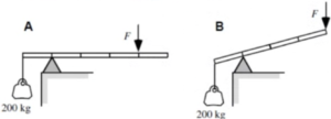
In both cases, a massless rod is supported by a fulcrum, and a \(200 \, \text{kg}\) hanging mass is suspended from the left end of the rod by a cable. A downward force \(F\) keeps the rod in rest. The rod in Case A is \(50 \, \text{cm}\) long, and the rod in Case B is \(40 \, \text{cm}\) long (each rod is marked at \(10 \, \text{cm}\) intervals). The magnitude of each vertical force \(F\) exerted on the rod will be
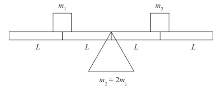
The system above is NOT balanced since \(m_2\) is twice the mass of \(m_1\). Which of the following changes would NOT balance the system so that there is 0 net torque? Assume the plank has no mass of its own.
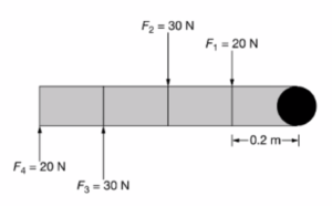
A rod may freely rotate about an axis that is perpendicular to the rod and is along the plane of the page. The rod is divided into four sections of equal length of 0.2 m each, and four forces are exerted on the rod, as shown in the figure. Frictional forces are considered negligible. Which of the following describes an additional torque that must be applied in order to keep the rod from rotating?


