(a) Calculate the linear speed of the sphere when it reaches the bottom of the incline.
| Step | Derivation/Formula | Reasoning |
|---|---|---|
| 1 | [katex]h = L \sin(\theta)[/katex] | Calculate the vertical height [katex]h[/katex] fallen by the sphere using the length of the incline [katex]L[/katex] and the sine of the incline angle [katex]\theta[/katex]. |
| 2 | [katex]h = 7.0 \sin(35^\circ)[/katex] | Substitute [katex]L = 7.0 \, m[/katex] and [katex]\theta = 35^\circ[/katex]. |
| 3 | [katex]PE_{\text{top}} = KE_{\text{trans}} + KE_{\text{rot}}[/katex] | Use the conservation of mechanical energy, where potential energy at the top is equal to the sum of transnational kinetic energy and rotational kinetic energy at the bottom. |
| 4 | [katex]mgh = \frac{1}{2}mv^2 + \frac{1}{2}I\omega^2[/katex] | Express the conservation of energy equation in terms of [katex]v[/katex] (linear velocity) and [katex]\omega[/katex] (angular velocity). |
| 5 | [katex]I = \frac{2}{5}MR^2[/katex] | Substitute the given moment of inertia for a solid sphere, where [katex]I = \frac{2}{5}MR^2[/katex]. |
| 6 | [katex]v = R\omega[/katex] | Relation between linear velocity and angular velocity for rolling without slipping. |
| 7 | [katex]\omega = \frac{v}{R}[/katex] | Rearrange the equation for [katex]\omega[/katex]. |
| 8 | [katex]mgh = \frac{1}{2}mv^2 + \frac{1}{2}(\frac{2}{5}MR^2)(\frac{v}{R})^2[/katex] | Substitute [katex]I[/katex] and [katex]\omega[/katex] in terms of [katex]v[/katex] and [katex]R[/katex]. |
| 9 | [katex]mgh = \frac{1}{2}mv^2 + \frac{1}{5}mv^2[/katex] | Simplify the equation by canceling [katex]M[/katex] and [katex]R[/katex]. |
| 10 | [katex]mgh = \frac{7}{10}mv^2[/katex] | Combine like terms. |
| 11 | [katex]v^2 = \frac{10}{7}gh[/katex] | Isolate [katex]v^2[/katex]. |
| 12 | [katex]v = \sqrt{\frac{10}{7}gh}[/katex] | Take the square root to find [katex]v[/katex]. |
| 13 | [katex]v = \sqrt{\frac{10}{7}(9.8)(7.0 \sin(35^\circ))}[/katex] | Substitute the values of [katex]g[/katex] and [katex]h[/katex]. |
| 14 | [katex]\boxed{v \approx 7.5 \, \text{m/s}}[/katex] | Final answer. |
(b) Determine the angular speed of the sphere at the bottom of the incline.
| Step | Derivation/Formula | Reasoning |
|---|---|---|
| 1 | [katex]\omega = \frac{v}{R}[/katex] | Use the relation between linear and angular velocities for a rolling object. |
| 2 | [katex]\omega = \frac{7.5}{0.15}[/katex] | Substitute [katex]v = 7.5 \, \text{m/s}[/katex] and [katex]R = 0.15 \, m[/katex] (converted from cm). |
| 3 | [katex]\boxed{\omega \approx 50 \, \text{rad/s}}[/katex] | Final answer. |
(c) Does the linear speed depend on the radius or mass of the sphere?
| Step | Analysis | Conclusion |
|---|---|---|
| 1 | From the energy conservation equation, the mass [katex]m[/katex] cancelled out and the final expression for [katex]v[/katex] didn’t include the radius [katex]R[/katex]. | The linear speed does not depend on the mass or radius of the sphere as both factors were eliminated in deriving [katex]v[/katex]. |
(d) Does the angular speed depend on the radius or mass of the sphere?
| Step | Analysis | Conclusion |
|---|---|---|
| 1 | Angular speed [katex]\omega[/katex] was found from [katex]v[/katex] divided by [katex]R[/katex], but it did not involve mass [katex]m[/katex]. | Angular speed does depend on the radius and does not depend on the mass of the sphere. |
A Major Upgrade To Phy Is Coming Soon — Stay Tuned
We'll help clarify entire units in one hour or less — guaranteed.
How long does it take for a rotating object to speed up from 15.0 rad/s to 33.3 rad/s if it has a uniform angular acceleration of 3.45 rad/s2?
An object’s angular momentum changes by \( 10 \,\text{kg} \cdot \text{m}^2/\text{s} \) in \( 2.0 \) \( \text{s} \). What magnitude average torque acted on this object?
A boy is sitting at a distance [katex] d_1 [/katex] from the fulcrum, and girl is sitting at a distance [katex] d_2 [/katex] from the fulcrum, with [katex] d_1 > d_2 [/katex]. The seesaw is level, with the two ends at the same height. Derive an equation for the minimum mass of the seesaw that will keep it balanced with the two children on it.
A solid ball and a cylinder roll down an inclined plane. Which reaches the bottom first?
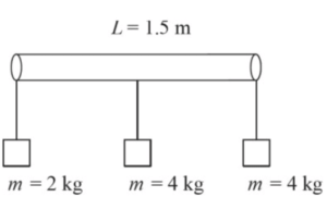
Three masses are attached to a \( 1.5 \, \text{m} \) long massless bar. Mass 1 is \( 2 \, \text{kg} \) and is attached to the far left side of the bar. Mass 2 is \( 4 \, \text{kg} \) and is attached to the far right side of the bar. Mass 3 is \( 4 \, \text{kg} \) and is attached to the middle of the bar. At what distance from the far left side of the bar can a string be attached to hold the bar up horizontally?
The angular velocity of an electric motor is \(\omega = \left(20 – \frac{1}{2} t^2 \right) \, \text{rad/s}\), where \(t\) is in seconds.
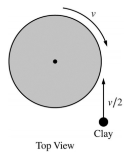
A system consists of a disk rotating on a frictionless axle and a piece of clay moving toward it, as shown in the figure above. The outside edge of the disk is moving at a linear speed \( v \), and the clay is moving at speed \( \frac{v}{2} \). The clay sticks to the outside edge of the disk. How does the angular momentum of the system after the clay sticks compare to the angular momentum of the system before the clay sticks, and what is an explanation for the comparison?
A turntable rotates through \( 6 \) \( \text{rad} \) in \( 3 \) \( \text{s} \) as it accelerates uniformly from rest. What is its angular acceleration in \( \text{rad/s}^2 \)?
When the speed of a rear-drive car is increasing on a horizontal road, what is the direction of the frictional force on the tires?
An ice skater performs a pirouette (a fast spin) by pulling in his outstretched arms close to his body. What happens to his angular momentum about the axis of rotation?
By continuing you (1) agree to our Terms of Use and Terms of Sale and (2) consent to sharing your IP and browser information used by this site’s security protocols as outlined in our Privacy Policy.
| Kinematics | Forces |
|---|---|
| \(\Delta x = v_i t + \frac{1}{2} at^2\) | \(F = ma\) |
| \(v = v_i + at\) | \(F_g = \frac{G m_1 m_2}{r^2}\) |
| \(v^2 = v_i^2 + 2a \Delta x\) | \(f = \mu N\) |
| \(\Delta x = \frac{v_i + v}{2} t\) | \(F_s =-kx\) |
| \(v^2 = v_f^2 \,-\, 2a \Delta x\) |
| Circular Motion | Energy |
|---|---|
| \(F_c = \frac{mv^2}{r}\) | \(KE = \frac{1}{2} mv^2\) |
| \(a_c = \frac{v^2}{r}\) | \(PE = mgh\) |
| \(T = 2\pi \sqrt{\frac{r}{g}}\) | \(KE_i + PE_i = KE_f + PE_f\) |
| \(W = Fd \cos\theta\) |
| Momentum | Torque and Rotations |
|---|---|
| \(p = mv\) | \(\tau = r \cdot F \cdot \sin(\theta)\) |
| \(J = \Delta p\) | \(I = \sum mr^2\) |
| \(p_i = p_f\) | \(L = I \cdot \omega\) |
| Simple Harmonic Motion | Fluids |
|---|---|
| \(F = -kx\) | \(P = \frac{F}{A}\) |
| \(T = 2\pi \sqrt{\frac{l}{g}}\) | \(P_{\text{total}} = P_{\text{atm}} + \rho gh\) |
| \(T = 2\pi \sqrt{\frac{m}{k}}\) | \(Q = Av\) |
| \(x(t) = A \cos(\omega t + \phi)\) | \(F_b = \rho V g\) |
| \(a = -\omega^2 x\) | \(A_1v_1 = A_2v_2\) |
| Constant | Description |
|---|---|
| [katex]g[/katex] | Acceleration due to gravity, typically [katex]9.8 , \text{m/s}^2[/katex] on Earth’s surface |
| [katex]G[/katex] | Universal Gravitational Constant, [katex]6.674 \times 10^{-11} , \text{N} \cdot \text{m}^2/\text{kg}^2[/katex] |
| [katex]\mu_k[/katex] and [katex]\mu_s[/katex] | Coefficients of kinetic ([katex]\mu_k[/katex]) and static ([katex]\mu_s[/katex]) friction, dimensionless. Static friction ([katex]\mu_s[/katex]) is usually greater than kinetic friction ([katex]\mu_k[/katex]) as it resists the start of motion. |
| [katex]k[/katex] | Spring constant, in [katex]\text{N/m}[/katex] |
| [katex] M_E = 5.972 \times 10^{24} , \text{kg} [/katex] | Mass of the Earth |
| [katex] M_M = 7.348 \times 10^{22} , \text{kg} [/katex] | Mass of the Moon |
| [katex] M_M = 1.989 \times 10^{30} , \text{kg} [/katex] | Mass of the Sun |
| Variable | SI Unit |
|---|---|
| [katex]s[/katex] (Displacement) | [katex]\text{meters (m)}[/katex] |
| [katex]v[/katex] (Velocity) | [katex]\text{meters per second (m/s)}[/katex] |
| [katex]a[/katex] (Acceleration) | [katex]\text{meters per second squared (m/s}^2\text{)}[/katex] |
| [katex]t[/katex] (Time) | [katex]\text{seconds (s)}[/katex] |
| [katex]m[/katex] (Mass) | [katex]\text{kilograms (kg)}[/katex] |
| Variable | Derived SI Unit |
|---|---|
| [katex]F[/katex] (Force) | [katex]\text{newtons (N)}[/katex] |
| [katex]E[/katex], [katex]PE[/katex], [katex]KE[/katex] (Energy, Potential Energy, Kinetic Energy) | [katex]\text{joules (J)}[/katex] |
| [katex]P[/katex] (Power) | [katex]\text{watts (W)}[/katex] |
| [katex]p[/katex] (Momentum) | [katex]\text{kilogram meters per second (kgm/s)}[/katex] |
| [katex]\omega[/katex] (Angular Velocity) | [katex]\text{radians per second (rad/s)}[/katex] |
| [katex]\tau[/katex] (Torque) | [katex]\text{newton meters (Nm)}[/katex] |
| [katex]I[/katex] (Moment of Inertia) | [katex]\text{kilogram meter squared (kgm}^2\text{)}[/katex] |
| [katex]f[/katex] (Frequency) | [katex]\text{hertz (Hz)}[/katex] |
Metric Prefixes
Example of using unit analysis: Convert 5 kilometers to millimeters.
Start with the given measurement: [katex]\text{5 km}[/katex]
Use the conversion factors for kilometers to meters and meters to millimeters: [katex]\text{5 km} \times \frac{10^3 \, \text{m}}{1 \, \text{km}} \times \frac{10^3 \, \text{mm}}{1 \, \text{m}}[/katex]
Perform the multiplication: [katex]\text{5 km} \times \frac{10^3 \, \text{m}}{1 \, \text{km}} \times \frac{10^3 \, \text{mm}}{1 \, \text{m}} = 5 \times 10^3 \times 10^3 \, \text{mm}[/katex]
Simplify to get the final answer: [katex]\boxed{5 \times 10^6 \, \text{mm}}[/katex]
Prefix | Symbol | Power of Ten | Equivalent |
|---|---|---|---|
Pico- | p | [katex]10^{-12}[/katex] | 0.000000000001 |
Nano- | n | [katex]10^{-9}[/katex] | 0.000000001 |
Micro- | µ | [katex]10^{-6}[/katex] | 0.000001 |
Milli- | m | [katex]10^{-3}[/katex] | 0.001 |
Centi- | c | [katex]10^{-2}[/katex] | 0.01 |
Deci- | d | [katex]10^{-1}[/katex] | 0.1 |
(Base unit) | – | [katex]10^{0}[/katex] | 1 |
Deca- or Deka- | da | [katex]10^{1}[/katex] | 10 |
Hecto- | h | [katex]10^{2}[/katex] | 100 |
Kilo- | k | [katex]10^{3}[/katex] | 1,000 |
Mega- | M | [katex]10^{6}[/katex] | 1,000,000 |
Giga- | G | [katex]10^{9}[/katex] | 1,000,000,000 |
Tera- | T | [katex]10^{12}[/katex] | 1,000,000,000,000 |
One price to unlock most advanced version of Phy across all our tools.
per month
Billed Monthly. Cancel Anytime.
We crafted THE Ultimate A.P Physics 1 Program so you can learn faster and score higher.
Try our free calculator to see what you need to get a 5 on the 2026 AP Physics 1 exam.
A quick explanation
Credits are used to grade your FRQs and GQs. Pro users get unlimited credits.
Submitting counts as 1 attempt.
Viewing answers or explanations count as a failed attempts.
Phy gives partial credit if needed
MCQs and GQs are are 1 point each. FRQs will state points for each part.
Phy customizes problem explanations based on what you struggle with. Just hit the explanation button to see.
Understand you mistakes quicker.

Phy automatically provides feedback so you can improve your responses.
10 Free Credits To Get You Started

By continuing you agree to nerd-notes.com Terms of Service, Privacy Policy, and our usage of user data.
Feeling uneasy about your next physics test? We'll boost your grade in 3 lessons or less—guaranteed

NEW! PHY AI accurately solves all questions
🔥 Get up to 30% off Elite Physics Tutoring
🧠 NEW! Learn Physics From Scratch Self Paced Course
🎯 Need exam style practice questions?
