# Part (a) Determine the sprinter’s constant acceleration during the first \(2 \, \text{seconds}\).
| Step | Derivation/Formula | Reasoning |
|---|---|---|
| 1 | [katex]d_1 = 100 \, \text{m} \, – \, 90 \, \text{m} = 10 \, \text{m}[/katex] | The first part of the sprint covers 10 meters. |
| 2 | [katex]d_1 = \frac{1}{2} a t_1^2[/katex] | Use the formula for distance under constant acceleration starting from rest: [katex]d = \frac{1}{2} a t^2[/katex]. |
| 3 | [katex]10 \, \text{m} = \frac{1}{2} a (2 \, \text{s})^2 [/katex] | Substitute [katex] d_1 = 10 \, \text{m} [/katex] and [katex] t_1 = 2 \, \text{s} [/katex]. |
| 4 | [katex]10 \, \text{m} = 2 a \, \text{s}^2 [/katex] | Simplify the equation. |
| 5 | [katex]a = 5 \, \text{m/s}^2 [/katex] | Solving for acceleration gives [katex]a[/katex]. |
| 6 | [katex]a = 5 \, \text{m/s}^2[/katex] | Constant acceleration value. |
# Part (b) Determine the sprinter’s velocity after 2 seconds have elapsed.
| Step | Derivation/Formula | Reasoning |
|---|---|---|
| 1 | [katex]v = a t_1 [/katex] | Using the formula for velocity under constant acceleration: [katex]v = a t[/katex]. |
| 2 | [katex]v = 5 \, \text{m/s}^2 \times 2 \, \text{s}[/katex] | Substitute [katex] a = 5 \, \text{m/s}^2 [/katex] and [katex] t_1 = 2 \, \text{s} [/katex]. |
| 3 | [katex]v = 10 \, \text{m/s}[/katex] | Solve for [katex]v[/katex]. |
# Part (c) Determine the total time needed to run the full 100 meters.
| Step | Derivation/Formula | Reasoning |
|---|---|---|
| 1 | [katex]v = d_2 / t_2 [/katex] | The velocity [katex]v[/katex] is constant for the remaining part of the race. |
| 2 | [katex]10 \, \text{m/s} = 90 \, \text{m} / t_2 [/katex] | Substitute [katex] v = 10 \, \text{m/s} [/katex] and [katex] d_2 = 90 \, \text{m} [/katex]. |
| 3 | [katex]t_2 = 90 \, \text{m} / 10 \, \text{m/s} [/katex] | Rearrange to solve for [katex] t_2 [/katex]. |
| 4 | [katex]t_2 = 9 \, \text{s} [/katex] | Solve for [katex] t_2 [/katex]. |
| 5 | [katex]t_{\text{total}} = t_1 + t_2 = 2 \, \text{s} + 9 \, \text{s} [/katex] | The total time is the sum of the two intervals. |
| 6 | [katex]t_{\text{total}} = 11 \, \text{s} [/katex] | Total time to run 100 meters. |
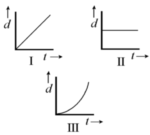
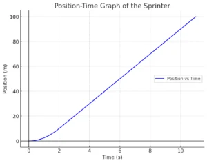
# Part (d) Draw the displacement vs time curve for the sprinter.
The displacement vs. time graph would show a parabolic curve for the first 2 seconds and a linear relationship thereafter to indicate constant velocity:
1. From [katex] t = 0 [/katex] to [katex] t = 2 [/katex] seconds, the curve will be a parabola opening upwards.
2. From [katex] t = 2[/katex] seconds to [katex] t = 11 [/katex] seconds, the curve will be a straight line with a constant slope of [katex]10 \, \text{m/s}[/katex].
A Major Upgrade To Phy Is Coming Soon — Stay Tuned
We'll help clarify entire units in one hour or less — guaranteed.
A car’s velocity increases as follows each second: \( 2 \) \( \text{m/s} \), \( 4 \) \( \text{m/s} \), \( 6 \) \( \text{m/s} \), \( 8 \) \( \text{m/s} \). This pattern shows that the car is:
In which of the following is the rate of change of the particle’s momentum zero?
A baseball is thrown vertically into the air with a velocity \( v \), and reaches a maximum height \( h \). At what height was the baseball moving with one-half its original velocity? Assume air resistance is negligible.
Which of the following graphs shows runners moving at the same speed? Assume the \(y\)-axis is measured in meters and the \(x\)-axis is measured in seconds.
A Corvette is traveling at a constant velocity \( 30 \, \text{m/s} \) when it passes a stationary supped up Civic. At that moment, the Civic puts the pedal to the floor and accelerates at \( 6 \, \text{m/s}^2 \). The Civic eventually catches up to the Corvette.
Which of the following graphs represent an object having zero acceleration?
An object undergoes constant acceleration. Starting from rest, the object travels \( 5 \, \text{m} \) in the first second. Then it travels \( 15 \, \text{m} \) in the next second. What total distance will be covered after the 3rd second?
A truck is traveling at \(35 \, \text{m/s}\) when the driver realizes the truck has no brakes. He sees a ramp off the road, inclined at \(20^\circ\), and decides to go up it to help the truck come to a stop. How far does the truck travel before coming to a stop (assume no friction)?
By continuing you (1) agree to our Terms of Use and Terms of Sale and (2) consent to sharing your IP and browser information used by this site’s security protocols as outlined in our Privacy Policy.
| Kinematics | Forces |
|---|---|
| \(\Delta x = v_i t + \frac{1}{2} at^2\) | \(F = ma\) |
| \(v = v_i + at\) | \(F_g = \frac{G m_1 m_2}{r^2}\) |
| \(v^2 = v_i^2 + 2a \Delta x\) | \(f = \mu N\) |
| \(\Delta x = \frac{v_i + v}{2} t\) | \(F_s =-kx\) |
| \(v^2 = v_f^2 \,-\, 2a \Delta x\) |
| Circular Motion | Energy |
|---|---|
| \(F_c = \frac{mv^2}{r}\) | \(KE = \frac{1}{2} mv^2\) |
| \(a_c = \frac{v^2}{r}\) | \(PE = mgh\) |
| \(T = 2\pi \sqrt{\frac{r}{g}}\) | \(KE_i + PE_i = KE_f + PE_f\) |
| \(W = Fd \cos\theta\) |
| Momentum | Torque and Rotations |
|---|---|
| \(p = mv\) | \(\tau = r \cdot F \cdot \sin(\theta)\) |
| \(J = \Delta p\) | \(I = \sum mr^2\) |
| \(p_i = p_f\) | \(L = I \cdot \omega\) |
| Simple Harmonic Motion | Fluids |
|---|---|
| \(F = -kx\) | \(P = \frac{F}{A}\) |
| \(T = 2\pi \sqrt{\frac{l}{g}}\) | \(P_{\text{total}} = P_{\text{atm}} + \rho gh\) |
| \(T = 2\pi \sqrt{\frac{m}{k}}\) | \(Q = Av\) |
| \(x(t) = A \cos(\omega t + \phi)\) | \(F_b = \rho V g\) |
| \(a = -\omega^2 x\) | \(A_1v_1 = A_2v_2\) |
| Constant | Description |
|---|---|
| [katex]g[/katex] | Acceleration due to gravity, typically [katex]9.8 , \text{m/s}^2[/katex] on Earth’s surface |
| [katex]G[/katex] | Universal Gravitational Constant, [katex]6.674 \times 10^{-11} , \text{N} \cdot \text{m}^2/\text{kg}^2[/katex] |
| [katex]\mu_k[/katex] and [katex]\mu_s[/katex] | Coefficients of kinetic ([katex]\mu_k[/katex]) and static ([katex]\mu_s[/katex]) friction, dimensionless. Static friction ([katex]\mu_s[/katex]) is usually greater than kinetic friction ([katex]\mu_k[/katex]) as it resists the start of motion. |
| [katex]k[/katex] | Spring constant, in [katex]\text{N/m}[/katex] |
| [katex] M_E = 5.972 \times 10^{24} , \text{kg} [/katex] | Mass of the Earth |
| [katex] M_M = 7.348 \times 10^{22} , \text{kg} [/katex] | Mass of the Moon |
| [katex] M_M = 1.989 \times 10^{30} , \text{kg} [/katex] | Mass of the Sun |
| Variable | SI Unit |
|---|---|
| [katex]s[/katex] (Displacement) | [katex]\text{meters (m)}[/katex] |
| [katex]v[/katex] (Velocity) | [katex]\text{meters per second (m/s)}[/katex] |
| [katex]a[/katex] (Acceleration) | [katex]\text{meters per second squared (m/s}^2\text{)}[/katex] |
| [katex]t[/katex] (Time) | [katex]\text{seconds (s)}[/katex] |
| [katex]m[/katex] (Mass) | [katex]\text{kilograms (kg)}[/katex] |
| Variable | Derived SI Unit |
|---|---|
| [katex]F[/katex] (Force) | [katex]\text{newtons (N)}[/katex] |
| [katex]E[/katex], [katex]PE[/katex], [katex]KE[/katex] (Energy, Potential Energy, Kinetic Energy) | [katex]\text{joules (J)}[/katex] |
| [katex]P[/katex] (Power) | [katex]\text{watts (W)}[/katex] |
| [katex]p[/katex] (Momentum) | [katex]\text{kilogram meters per second (kgm/s)}[/katex] |
| [katex]\omega[/katex] (Angular Velocity) | [katex]\text{radians per second (rad/s)}[/katex] |
| [katex]\tau[/katex] (Torque) | [katex]\text{newton meters (Nm)}[/katex] |
| [katex]I[/katex] (Moment of Inertia) | [katex]\text{kilogram meter squared (kgm}^2\text{)}[/katex] |
| [katex]f[/katex] (Frequency) | [katex]\text{hertz (Hz)}[/katex] |
Metric Prefixes
Example of using unit analysis: Convert 5 kilometers to millimeters.
Start with the given measurement: [katex]\text{5 km}[/katex]
Use the conversion factors for kilometers to meters and meters to millimeters: [katex]\text{5 km} \times \frac{10^3 \, \text{m}}{1 \, \text{km}} \times \frac{10^3 \, \text{mm}}{1 \, \text{m}}[/katex]
Perform the multiplication: [katex]\text{5 km} \times \frac{10^3 \, \text{m}}{1 \, \text{km}} \times \frac{10^3 \, \text{mm}}{1 \, \text{m}} = 5 \times 10^3 \times 10^3 \, \text{mm}[/katex]
Simplify to get the final answer: [katex]\boxed{5 \times 10^6 \, \text{mm}}[/katex]
Prefix | Symbol | Power of Ten | Equivalent |
|---|---|---|---|
Pico- | p | [katex]10^{-12}[/katex] | 0.000000000001 |
Nano- | n | [katex]10^{-9}[/katex] | 0.000000001 |
Micro- | µ | [katex]10^{-6}[/katex] | 0.000001 |
Milli- | m | [katex]10^{-3}[/katex] | 0.001 |
Centi- | c | [katex]10^{-2}[/katex] | 0.01 |
Deci- | d | [katex]10^{-1}[/katex] | 0.1 |
(Base unit) | – | [katex]10^{0}[/katex] | 1 |
Deca- or Deka- | da | [katex]10^{1}[/katex] | 10 |
Hecto- | h | [katex]10^{2}[/katex] | 100 |
Kilo- | k | [katex]10^{3}[/katex] | 1,000 |
Mega- | M | [katex]10^{6}[/katex] | 1,000,000 |
Giga- | G | [katex]10^{9}[/katex] | 1,000,000,000 |
Tera- | T | [katex]10^{12}[/katex] | 1,000,000,000,000 |
One price to unlock most advanced version of Phy across all our tools.
per month
Billed Monthly. Cancel Anytime.
We crafted THE Ultimate A.P Physics 1 Program so you can learn faster and score higher.
Try our free calculator to see what you need to get a 5 on the 2026 AP Physics 1 exam.
A quick explanation
Credits are used to grade your FRQs and GQs. Pro users get unlimited credits.
Submitting counts as 1 attempt.
Viewing answers or explanations count as a failed attempts.
Phy gives partial credit if needed
MCQs and GQs are are 1 point each. FRQs will state points for each part.
Phy customizes problem explanations based on what you struggle with. Just hit the explanation button to see.
Understand you mistakes quicker.

Phy automatically provides feedback so you can improve your responses.
10 Free Credits To Get You Started

By continuing you agree to nerd-notes.com Terms of Service, Privacy Policy, and our usage of user data.
Feeling uneasy about your next physics test? We'll boost your grade in 3 lessons or less—guaranteed

NEW! PHY AI accurately solves all questions
🔥 Get up to 30% off Elite Physics Tutoring
🧠 NEW! Learn Physics From Scratch Self Paced Course
🎯 Need exam style practice questions?
