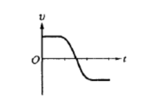
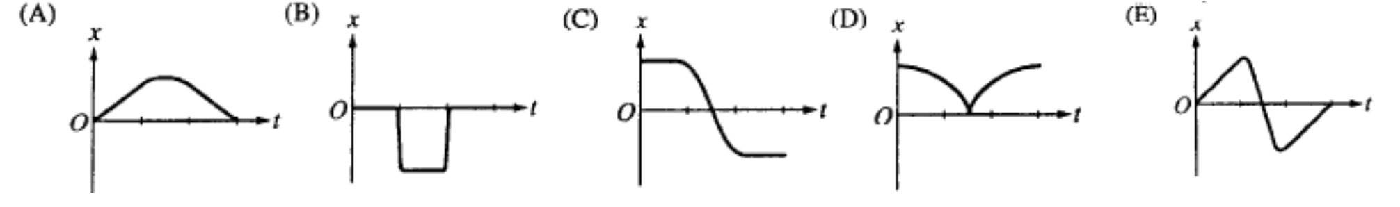
The graph above shows velocity \( v \) versus time \( t \) for an object in linear motion. Which of the following is a possible graph of position (\( x \)) versus time (\( t \)) for this object?
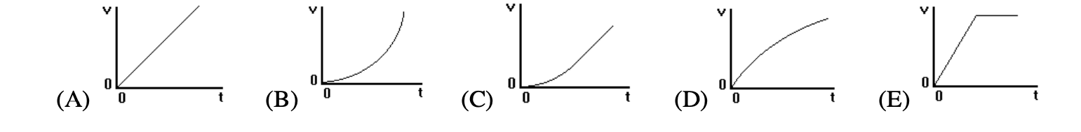
A large beach ball is dropped from the ceiling of a school gymnasium to the floor about 10 meters below. Which of the following graphs would best represent its velocity as a function of time? (do not neglect air resistance)
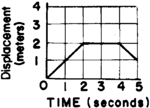
The graph above represents the motion of an object traveling in a straight line as a function of time. What is the average speed of the object during the first four seconds?
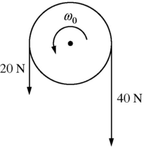
A disk is initially rotating counterclockwise around a fixed axis with angular speed \( \omega_0 \). At time \( t = 0 \), the two forces shown in the figure above are exerted on the disk. If counterclockwise is positive, which of the following could show the angular velocity of the disk as a function of time?
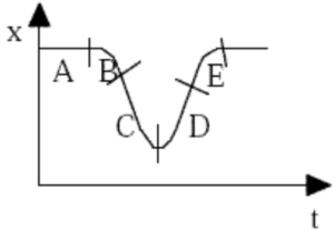 The graph below is a plot of position versus time. For which labeled segments is the velocity positive and the acceleration negative?
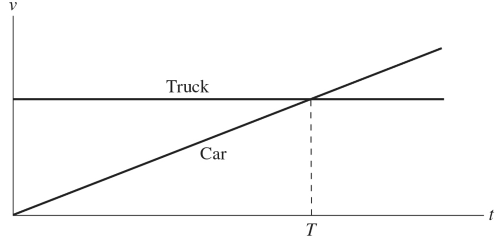
The motions of a car and a truck along a straight road are represented by the velocity–time graphs in the figure. The two vehicles are initially alongside each other at time \(t = 0\). At time \(T\), what is true of the distances traveled by the vehicles since time \(t = 0\)?
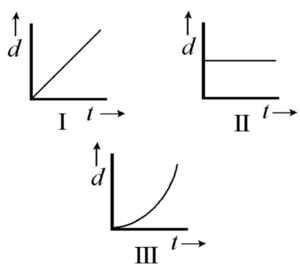 In which of the following is the particle’s acceleration constant?
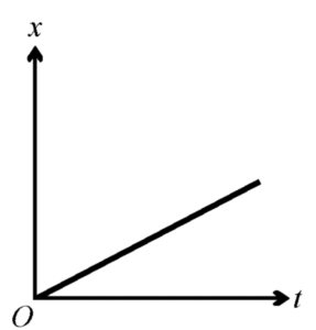 The displacement \(x\) of an object moving in one dimension is shown above as a function of time \(t\). The velocity of this object must be
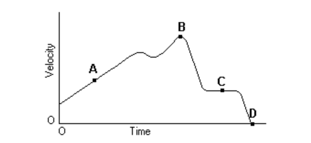 Above is the graph of the velocity vs. time of a duck flying due south for the winter. At what point might the duck begin reversing directions?


