
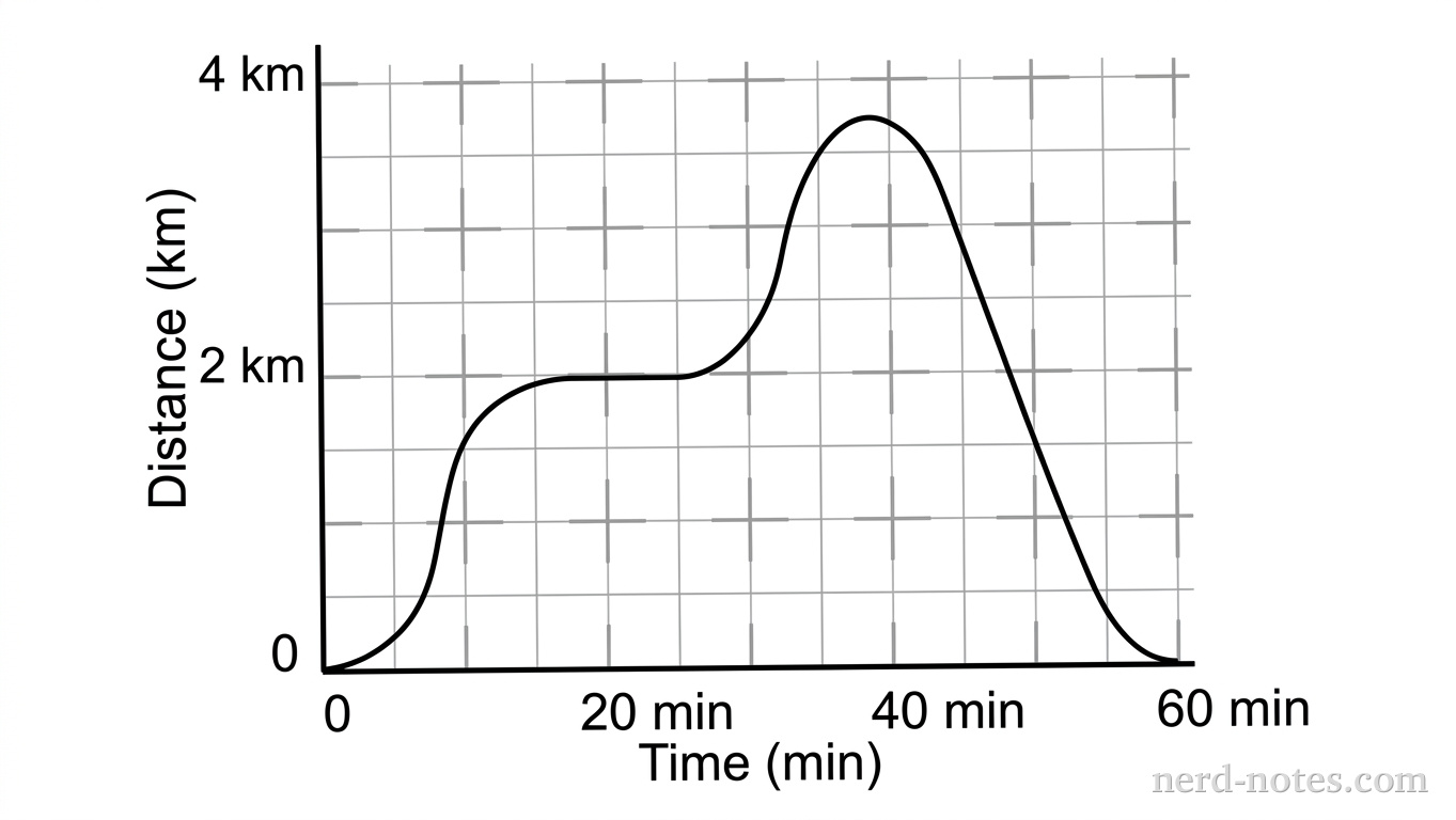
Above is a graph of the \(distance\) vs. time for car moving along a road. According the graph, at which of the following times would the automobile have been accelerating positively?
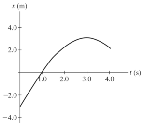
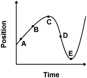
The graph in the figure shows the position of a particle as it travels along the x-axis. At what value of \(t\) is the speed of the particle equal to \(0 \, \text{m/s}\)?
note that the slope of position vs time is velocity. And the graph most closely reemsbles a flat or 0 slope at 3 seconds
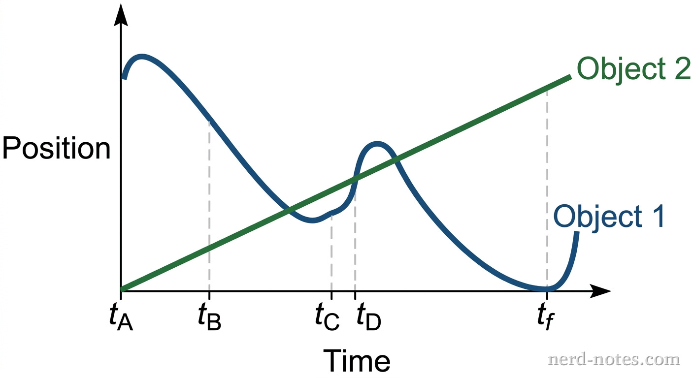
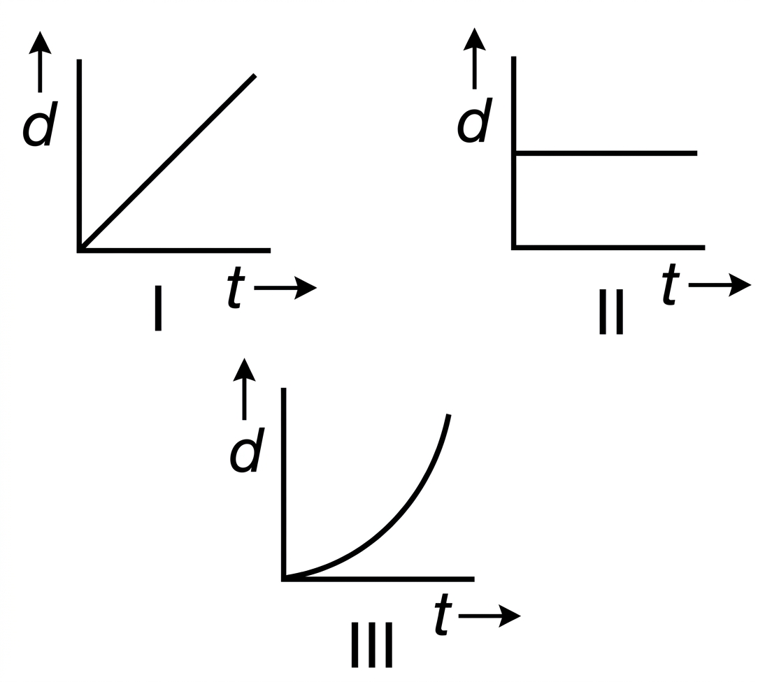
Which statement is true about the distances the two objects have traveled at time \( t_f \)?
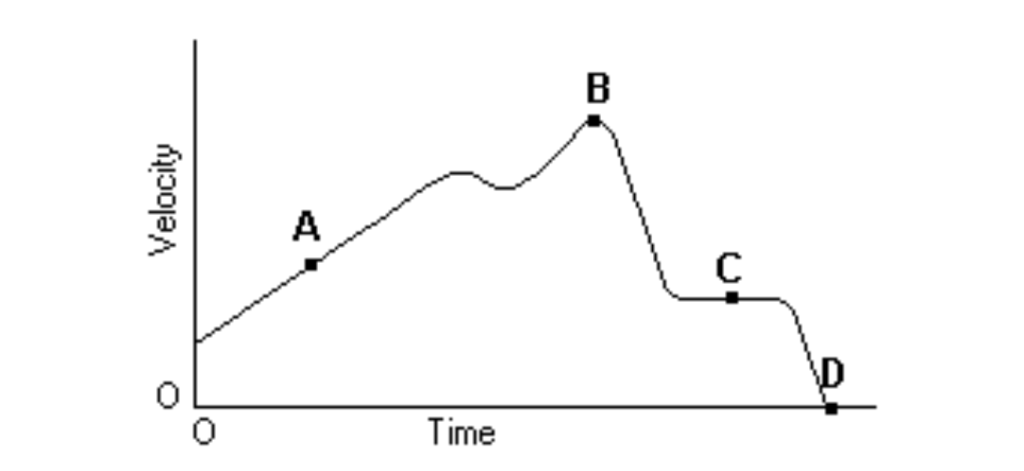 Above is the graph of the velocity vs. time of a duck flying due south for the winter. At what point might the duck begin reversing directions?
 Based on this graph…
 In which of the following is the particle’s acceleration constant?

A \( 0.20 \) \( \text{kg} \) object moves along a straight line. The net force acting on the object varies with the object’s displacement as shown in the graph above. The object starts from rest at displacement \( x = 0 \) and time \( t = 0 \) and is displaced a distance of \( 20 \) \( \text{m} \). Determine each of the following.


