| Step | Derivation/Formula | Reasoning |
|---|---|---|
| 1 | \[ \Delta L = \int_{0}^{6} \tau(t)\,dt \] | This is the fundamental relation in rotational dynamics stating that the change in angular momentum \(\Delta L\) is the time-integral (area under the curve) of the net torque \(\tau\) from \(t = 0\) to \(t = 6\) seconds. |
| 2 | \(\tau\ \text{vs.}\ t\ \text{graph}\) | The table provides net torque values at different times; plotting these yields a straight line indicating a linear increase in torque with time. |
| 3 | \(\tau(0) = 0,\; \tau(2) = 1.5,\; \tau(4) = 3.0,\; \tau(6) = 4.5\ \text{(in N\cdot m)}\) | The data shows that the net torque increases uniformly, so the graph from \(t=0\) to \(t=6\) seconds forms a right triangle. |
| 4 | \( \Delta L = \frac{1}{2}\,(\Delta t)\,(\tau_{\text{max}}) \) | Since the net torque increases linearly, the area under the \(\tau\) vs. \(t\) graph (which equals \(\Delta L\)) is the area of a triangle with base \(\Delta t = 6\) s and height \(\tau_{\text{max}} = 4.5\ \text{N\cdot m}\). |
| 5 | \( \Delta L = \frac{1}{2} \times 6\,\text{s} \times 4.5\,\text{N\cdot m} = 13.5\,\text{N\cdot m\cdot s} \) | This calculation gives the numerical value of the change in angular momentum over the 6-second interval. |
| 6 | Option (d): Graph the net torque vs. time and find the area under the curve. | This is the correct method because the area under the \(\tau\) vs. \(t\) graph directly represents the change in angular momentum \(\Delta L\), as derived above. |
| 7 | Incorrect Options: | – Option (a) incorrectly multiplies the maximum torque by the total time, ignoring that the torque is not constant. – Option (b) incorrectly divides the maximum torque by time. – Option (c) finds the slope, which does not yield the change in momentum because the slope represents the rate of change of torque, not the integrated effect over time. |
| 8 | \( \boxed{\Delta L = 13.5\,\text{N\cdot m\cdot s}} \) | This boxed result is the final change in angular momentum and confirms that option (d) is the proper procedure to use the data table. |
A Major Upgrade To Phy Is Coming Soon — Stay Tuned
We'll help clarify entire units in one hour or less — guaranteed.
A 0.72-m-diameter solid sphere can be rotated about an axis through its center by a torque of 10.8 N·m which accelerates it uniformly from rest through a total of 160 revolutions in 15.0 s. What is the mass of the sphere?
A boy and a girl are balanced on a massless seesaw. The boy has a mass of \(60 \, \text{kg}\) and the girl’s mass is \(50 \, \text{kg}\). If the boy sits \(1.5 \, \text{m}\) from the pivot point on one side of the seesaw, where must the girl sit on the other side for equilibrium?
Two equal-magnitude forces are applied to a door at the doorknob. The first force is applied perpendicular to the door, and the second force is applied at \( 30^\circ \) to the plane of the door. Which force exerts the greater torque about the door hinge?
A ladder at rest is leaning against a wall at an angle. Which of the following forces must have the same magnitude as the frictional force exerted on the ladder by the floor?
Two forces produce equal torques on a door about the door hinge. The first force is applied at the midpoint of the door; the second force is applied at the doorknob. Both forces are applied perpendicular to the door. Which force has a greater magnitude?
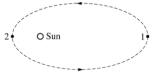
The elliptical orbit of a comet is shown above. Positions 1 and 2 are, respectively, the farthest and nearest positions to the Sun, and at position 1 the distance from the comet to the Sun is 10 times that at position 2. What is the ratio \(v_1\)/\(v_2\) of the speed of the comet at position 1 to the speed at position 2?
A \( 0.72 \) \( \text{m} \)-diameter solid sphere can be rotated about an axis through its center by a torque of \( 10.8 \) \( \text{Nm} \) which accelerates it uniformly from rest through a total of \( 160 \) revolutions in \( 15.0 \) \( \text{s} \). What is the mass of the sphere?
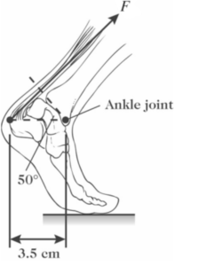
The figure shows a person’s foot. In that figure, the Achilles tendon exerts a force of magnitude F = 720 N. What is the magnitude of the torque that this force produces about the ankle joint?
A solid metal bar is at rest on a horizontal frictionless surface. It is free to rotate about a vertical axis at the left end. The figures below show forces of different magnitudes that are exerted on the bar at different locations. In which case does the bar’s angular speed about the axis increase at the fastest rate?
A student is asked to design an experiment to determine the change in angular momentum of a disk that rotates about its center and the product of the average torque applied to the disk and the time interval in which the torque is exerted. A net force is applied tangentially to the surface of the disk. The rotational inertia of the disk about its center is [katex]I = MR^2[/katex]. Which two of the following quantities should the student measure to determine the change in angular momentum of the disk after 10 s? Select two answers.
\( \boxed{\Delta L = 13.5\,\text{N\cdot m\cdot s}} \)
By continuing you (1) agree to our Terms of Use and Terms of Sale and (2) consent to sharing your IP and browser information used by this site’s security protocols as outlined in our Privacy Policy.
| Kinematics | Forces |
|---|---|
| \(\Delta x = v_i t + \frac{1}{2} at^2\) | \(F = ma\) |
| \(v = v_i + at\) | \(F_g = \frac{G m_1 m_2}{r^2}\) |
| \(v^2 = v_i^2 + 2a \Delta x\) | \(f = \mu N\) |
| \(\Delta x = \frac{v_i + v}{2} t\) | \(F_s =-kx\) |
| \(v^2 = v_f^2 \,-\, 2a \Delta x\) |
| Circular Motion | Energy |
|---|---|
| \(F_c = \frac{mv^2}{r}\) | \(KE = \frac{1}{2} mv^2\) |
| \(a_c = \frac{v^2}{r}\) | \(PE = mgh\) |
| \(T = 2\pi \sqrt{\frac{r}{g}}\) | \(KE_i + PE_i = KE_f + PE_f\) |
| \(W = Fd \cos\theta\) |
| Momentum | Torque and Rotations |
|---|---|
| \(p = mv\) | \(\tau = r \cdot F \cdot \sin(\theta)\) |
| \(J = \Delta p\) | \(I = \sum mr^2\) |
| \(p_i = p_f\) | \(L = I \cdot \omega\) |
| Simple Harmonic Motion | Fluids |
|---|---|
| \(F = -kx\) | \(P = \frac{F}{A}\) |
| \(T = 2\pi \sqrt{\frac{l}{g}}\) | \(P_{\text{total}} = P_{\text{atm}} + \rho gh\) |
| \(T = 2\pi \sqrt{\frac{m}{k}}\) | \(Q = Av\) |
| \(x(t) = A \cos(\omega t + \phi)\) | \(F_b = \rho V g\) |
| \(a = -\omega^2 x\) | \(A_1v_1 = A_2v_2\) |
| Constant | Description |
|---|---|
| [katex]g[/katex] | Acceleration due to gravity, typically [katex]9.8 , \text{m/s}^2[/katex] on Earth’s surface |
| [katex]G[/katex] | Universal Gravitational Constant, [katex]6.674 \times 10^{-11} , \text{N} \cdot \text{m}^2/\text{kg}^2[/katex] |
| [katex]\mu_k[/katex] and [katex]\mu_s[/katex] | Coefficients of kinetic ([katex]\mu_k[/katex]) and static ([katex]\mu_s[/katex]) friction, dimensionless. Static friction ([katex]\mu_s[/katex]) is usually greater than kinetic friction ([katex]\mu_k[/katex]) as it resists the start of motion. |
| [katex]k[/katex] | Spring constant, in [katex]\text{N/m}[/katex] |
| [katex] M_E = 5.972 \times 10^{24} , \text{kg} [/katex] | Mass of the Earth |
| [katex] M_M = 7.348 \times 10^{22} , \text{kg} [/katex] | Mass of the Moon |
| [katex] M_M = 1.989 \times 10^{30} , \text{kg} [/katex] | Mass of the Sun |
| Variable | SI Unit |
|---|---|
| [katex]s[/katex] (Displacement) | [katex]\text{meters (m)}[/katex] |
| [katex]v[/katex] (Velocity) | [katex]\text{meters per second (m/s)}[/katex] |
| [katex]a[/katex] (Acceleration) | [katex]\text{meters per second squared (m/s}^2\text{)}[/katex] |
| [katex]t[/katex] (Time) | [katex]\text{seconds (s)}[/katex] |
| [katex]m[/katex] (Mass) | [katex]\text{kilograms (kg)}[/katex] |
| Variable | Derived SI Unit |
|---|---|
| [katex]F[/katex] (Force) | [katex]\text{newtons (N)}[/katex] |
| [katex]E[/katex], [katex]PE[/katex], [katex]KE[/katex] (Energy, Potential Energy, Kinetic Energy) | [katex]\text{joules (J)}[/katex] |
| [katex]P[/katex] (Power) | [katex]\text{watts (W)}[/katex] |
| [katex]p[/katex] (Momentum) | [katex]\text{kilogram meters per second (kgm/s)}[/katex] |
| [katex]\omega[/katex] (Angular Velocity) | [katex]\text{radians per second (rad/s)}[/katex] |
| [katex]\tau[/katex] (Torque) | [katex]\text{newton meters (Nm)}[/katex] |
| [katex]I[/katex] (Moment of Inertia) | [katex]\text{kilogram meter squared (kgm}^2\text{)}[/katex] |
| [katex]f[/katex] (Frequency) | [katex]\text{hertz (Hz)}[/katex] |
Metric Prefixes
Example of using unit analysis: Convert 5 kilometers to millimeters.
Start with the given measurement: [katex]\text{5 km}[/katex]
Use the conversion factors for kilometers to meters and meters to millimeters: [katex]\text{5 km} \times \frac{10^3 \, \text{m}}{1 \, \text{km}} \times \frac{10^3 \, \text{mm}}{1 \, \text{m}}[/katex]
Perform the multiplication: [katex]\text{5 km} \times \frac{10^3 \, \text{m}}{1 \, \text{km}} \times \frac{10^3 \, \text{mm}}{1 \, \text{m}} = 5 \times 10^3 \times 10^3 \, \text{mm}[/katex]
Simplify to get the final answer: [katex]\boxed{5 \times 10^6 \, \text{mm}}[/katex]
Prefix | Symbol | Power of Ten | Equivalent |
|---|---|---|---|
Pico- | p | [katex]10^{-12}[/katex] | 0.000000000001 |
Nano- | n | [katex]10^{-9}[/katex] | 0.000000001 |
Micro- | µ | [katex]10^{-6}[/katex] | 0.000001 |
Milli- | m | [katex]10^{-3}[/katex] | 0.001 |
Centi- | c | [katex]10^{-2}[/katex] | 0.01 |
Deci- | d | [katex]10^{-1}[/katex] | 0.1 |
(Base unit) | – | [katex]10^{0}[/katex] | 1 |
Deca- or Deka- | da | [katex]10^{1}[/katex] | 10 |
Hecto- | h | [katex]10^{2}[/katex] | 100 |
Kilo- | k | [katex]10^{3}[/katex] | 1,000 |
Mega- | M | [katex]10^{6}[/katex] | 1,000,000 |
Giga- | G | [katex]10^{9}[/katex] | 1,000,000,000 |
Tera- | T | [katex]10^{12}[/katex] | 1,000,000,000,000 |
One price to unlock most advanced version of Phy across all our tools.
per month
Billed Monthly. Cancel Anytime.
We crafted THE Ultimate A.P Physics 1 Program so you can learn faster and score higher.
Try our free calculator to see what you need to get a 5 on the 2026 AP Physics 1 exam.
A quick explanation
Credits are used to grade your FRQs and GQs. Pro users get unlimited credits.
Submitting counts as 1 attempt.
Viewing answers or explanations count as a failed attempts.
Phy gives partial credit if needed
MCQs and GQs are are 1 point each. FRQs will state points for each part.
Phy customizes problem explanations based on what you struggle with. Just hit the explanation button to see.
Understand you mistakes quicker.

Phy automatically provides feedback so you can improve your responses.
10 Free Credits To Get You Started

By continuing you agree to nerd-notes.com Terms of Service, Privacy Policy, and our usage of user data.
Feeling uneasy about your next physics test? We'll boost your grade in 3 lessons or less—guaranteed

NEW! PHY AI accurately solves all questions
🔥 Get up to 30% off Elite Physics Tutoring
🧠 NEW! Learn Physics From Scratch Self Paced Course
🎯 Need exam style practice questions?
