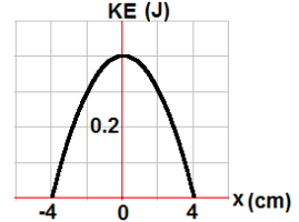
A 0.2 kg object is attached to a horizontal spring undergoes SHM with the total energy of 0.4 J. The kinetic energy as a function of position presented by the graph.
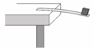
Students attach a thin strip of metal to a table so that the strip is horizontal in relation to the ground. A section of the strip hangs off the edge of the table. A mass is secured to the end of the hanging section of the strip and is then displaced so that the mass-strip system oscillates, as shown in the figure. Students make various measurements of the net force F exerted on the mass as a result of the force due to gravity and the normal force from the strip, the vertical position y of the mass above and below its equilibrium position y. and the period of oscillation T’ when the mass is displaced by different amplitudes A. Which of the following explanations is correct about the evidence required to conclude that the mass undergoes simple harmonic motion?
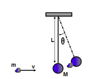
A \(20 \, \text{g}\) piece of clay moving at a speed of \(50 \, \text{m/s}\) strikes a \(500 \, \text{g}\) pendulum bob at rest. The length of a string is \(0.8 \, \text{m}\). After the collision, the clay-bob system starts to oscillate as a simple pendulum.
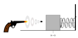
A bullet (mass: \(0.05 \, \text{kg}\)) is fired horizontally (\(v = 200 \, \text{m/s}\)) at a block (mass: \(1.3 \, \text{kg}\)) initially at rest on a frictionless surface. The block is attached to a spring (\(k = 2500 \, \text{N/m}\)). The bullet becomes embedded. Calculate:


