A flat rectangular loop of wire with length $L$, width $w$, and resistance $R$ moves in the $+x$-direction at constant speed $v_0$. At time $t = 0$, the front edge of the loop enters a magnetic field region extending from $x = 0$ to $x = 2L$. Within this region, the magnetic field is directed into the page with spatially varying magnitude $B(x) = B_0 \dfrac{x}{L}$, where $B_0$ is a positive constant, and $B = 0$ elsewhere. Defining counterclockwise current as positive, the induced current $I(t)$ as a function of time increases linearly from $0$ to $+I_0$ for $0 \le t \le T$, remains constant at $+I_0$ for $T \le t \le 2T$, and jumps to $-I_0$ at $t = 2T$ before rising linearly to $0$ at $t = 3T$, where $T = \dfrac{L}{v_0}$ and $I_0 = \dfrac{B_0 w v_0}{R}$. Which of the following claims correctly explains the physical origin of a feature in the $I(t)$ graph? • Nerd Notes

AP Physics

Unit 1 - Vectors and Kinematics

MCQ

Mathematical

Advanced

Step	Reasoning
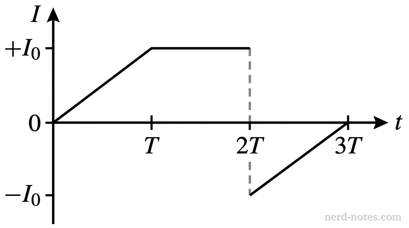
Identify the target principle for induced current in terms of magnetic flux rate of change and motional EMF. \[ I(t) = \dfrac{\mathcal{E}_{\text{net}}}{R} = \dfrac{1}{R} \left\| \dfrac{d\Phi_B}{dt} \right\| \]	The question asks for the physical origin of the constant current plateau $+I_0$ during the interval $T < t < 2T$.
Calculate the magnetic flux $\Phi_B(t)$ through the loop when it is entirely inside the field region $0 \le x \le 2L$. \[ \Phi_B(t) = \int_{v_0 t – L}^{v_0 t} \left( B_0 \dfrac{x}{L} \right) w \, dx = \dfrac{B_0 w}{2L} \left[ (v_0 t)^2 – (v_0 t – L)^2 \right] = B_0 w v_0 t – \dfrac{1}{2} B_0 w L \]	During $T \le t \le 2T$, the front edge is at position $x_f = v_0 t$ and the rear edge is at $x_b = v_0 t – L$. Integrating $B(x) = B_0 \dfrac{x}{L}$ over the loop length yields the enclosed flux.
Differentiate the flux with respect to time to find the net induced EMF and current during this interval. \[ \mathcal{E} = \dfrac{d\Phi_B}{dt} = B_0 w v_0 \implies I = \dfrac{B_0 w v_0}{R} = +I_0 \]	Faraday’s law connects the time derivative of magnetic flux to the induced EMF.
Relate the constant net EMF to the motional EMF along the leading and trailing edges of the loop. \[ \mathcal{E}_{\text{net}} = \mathcal{E}_f – \mathcal{E}_b = [B(x_f) – B(x_b)] w v_0 = \left[ B_0 \dfrac{v_0 t}{L} – B_0 \dfrac{v_0 t – L}{L} \right] w v_0 = B_0 w v_0 \]	Motional EMF provides an equivalent physical framework: the leading edge experiences an upward EMF $\mathcal{E}_f = B(x_f) w v_0$ and the trailing edge experiences an upward EMF $\mathcal{E}_b = B(x_b) w v_0$.
Conclude why the difference in magnetic field strength produces the constant plateau.	Because the spatial field gradient $\dfrac{dB}{dx} = \dfrac{B_0}{L}$ is constant, the difference in magnetic field strength between the front and rear edges separated by distance $L$ is strictly constant: $\Delta B = B_0$. This produces a constant net motional EMF $\mathcal{E}_{\text{net}} = B_0 w v_0$ and a constant current $+I_0$.

Why each choice is correct or incorrect:

(A) Incorrect. Magnetic flux increases continuously at a rate of $\dfrac{d\Phi_B}{dt} = B_0 w v_0$ because the loop moves into regions of higher field strength.

(B) Incorrect. A constant rate of area increase in a uniform field yields a constant current; here, current increases linearly because $B(x)$ varies linearly with position, making $\Phi_B \propto t^2$ and $I \propto t$.

(C) Incorrect. The magnetic field vector points into the page everywhere in the region; the current reverses direction because flux changes from increasing to decreasing as the loop exits.

(D) This is the correct answer. The constant field difference $\Delta B = B_0$ between the leading and trailing edges produces a constant net motional EMF $\mathcal{E}_{\text{net}} = B_0 w v_0$.

Need Help? Ask Phy To Explain

A Major Upgrade To Phy Is Coming Soon — Stay Tuned

Just Drag and Drop!

Quick Actions ?

NEW UBQ QUIZ LAB

100s of AP aligned questions and quizzes to help you get a 5 even faster. Full Mock exams with Auto Grading and Adaptive explanations. Try out Nerd Notes', state of the art, quiz platform.

Topics in this question

Need 1 to 1 Help? Book a trial lesson here.

We'll help clarify entire units in one hour or less — guaranteed.

Need to Learn AP Physics From Scratch Quickly? We have Program for that.

A self paced course with videos, problems sets, and everything you need to get a 5. Trusted by over 15k students and over 200 schools.

Go Pro to remove ads + unlimited access to our AI learning tools.

Related Questions

5 More similar questions to the one you just solved

Intermediate

Mathematical

MCQ

$A Cartesian graph plotting induced EMF \mathcal{E} on the vertical axis against time t on the horizontal axis. The vertical axis is labeled \mathcal{E} at the top and has tick marks at \mathcal{E}_0, 0, and -\mathcal{E}_0. The horizontal axis is labeled t at the far right and has tick marks at 0, T, 2T, and 3T. From t = 0 to t = T, a horizontal solid line segment lies at \mathcal{E} = -\mathcal{E}_0. From t = T to t = 2T, a horizontal solid line segment lies along the horizontal axis at \mathcal{E} = 0. From t = 2T to t = 3T, a horizontal solid line segment lies at \mathcal{E} = +\mathcal{E}_0. Vertical dashed line segments connect (T, -\mathcal{E}_0) to (T, 0) and (2T, 0) to (2T, \mathcal{E}_0). No other labels or lines appear.$

A conducting loop is fixed in a region with a magnetic field directed perpendicular to the plane of the loop. The induced electromotive force (EMF) $\mathcal{E}$ in the loop is measured as a function of time $t$ and is shown in the graph. At time $t = 0$, the magnetic flux through the loop is zero ($\Phi_B = 0$). Which of the following graphs best represents the magnetic flux $\Phi_B$ through the loop as a function of time $t$?

Intermediate

Mathematical

MCQ

A rigid circular wire loop of radius $a$ and total resistance $R$ lies fixed in a plane perpendicular to a spatially uniform magnetic field. The magnitude of the magnetic field changes with time $t$ according to $B(t) = B_0 \left(1 + \dfrac{t}{\tau}\right)^3$, where $B_0$ and $\tau$ are positive constants. Which of the following expressions represents the total electric charge $Q$ that flows past a point in the loop between $t = 0$ and $t = \tau$?

Beginner

Mathematical

MCQ

An ideal circuit consists of an inductor of inductance $L$ connected in series with a capacitor of capacitance $C$. At time $t = 0$, the capacitor carries an initial charge $Q_0$ and the current in the circuit is zero. Which of the following graphs best represents the charge $q(t)$ on the capacitor as a function of time $t$?

Intermediate

Mathematical

MCQ

$A 3D Cartesian coordinate system with x, y, and z axes labeled at the ends of thin black lines with arrowheads. A flat square loop of side length L is situated in the xy-plane with one edge lying along the y-axis from y = 0 to y = L. A second identical square loop shares the same edge along the y-axis but is tilted upward into the xz-plane by an angle \theta relative to the xy-plane. An arc labeled \theta indicates the tilt angle between the two loop planes. Vertical upward arrows parallel to the z-axis represent a magnetic field \vec{B}; the arrows increase in length at larger values of x. No other labels, lines, text, or axes appear.$

A square loop of wire with side length $L$ lies in a region containing a non-uniform magnetic field $\vec{B} = B_0 \left(\dfrac{x}{L}\right) \hat{k}$, where $B_0$ is a positive constant and $x \ge 0$. One edge of the loop is fixed along the $y$-axis from $y = 0$ to $y = L$. The loop is tilted about the $y$-axis by an angle $\theta$ relative to the $xy$-plane. What is the ratio of the magnetic flux through the loop when $\theta = 60^\circ$ to the magnetic flux through the loop when $\theta = 0^\circ$?

Advanced

Mathematical

MCQ

A horizontal circular ring of radius $r$, mass $m$, and electrical resistance $R$ falls vertically under the influence of gravity through a region with a non-uniform vertical magnetic field. The vertical component of the magnetic field varies linearly with height $z$ according to $B_z(z) = B_0 + bz$, where $B_0$ and $b$ are positive constants, and $z$ is measured upward. Air resistance is negligible. Which of the following expressions correctly represents the magnitude of the ring’s terminal velocity $v_T$?

Advanced

Mathematical

MCQ

$A circular conducting disk of radius R lies flat in the xy-plane, centered at the origin. A vertical z-axis extends upward through the center of the disk, with a curved arrow around the z-axis indicating rotation at constant angular velocity \omega. A radial line segment extends from the origin to the outer rim of the disk, labeled R. Several upward-pointing magnetic field vectors \vec{B}(r) pass vertically through the disk, with shorter vectors near the center and longer vectors near the outer rim to represent the radial increase in field magnitude. No other labels, lines, text, or axes appear.$

A thin, uniform conducting disk of radius $R$ rotates in the $xy$-plane about a fixed vertical axis through its center with a constant angular speed $\omega$. A non-uniform magnetic field perpendicular to the plane of the disk is given by $\vec{B}(r) = B_0 \left(\dfrac{r}{R}\right)^2 \hat{k}$, where $r$ is the radial distance from the axis of rotation and $B_0$ is a positive constant. Which of the following expressions represents the magnitude of the induced electromotive force (EMF) between the center of the disk and its outer rim?

Advanced

Mathematical

MCQ

A long, straight cylindrical wire of radius $R$ carries a steady total current $I$ distributed uniformly across its circular cross section. The permeability of free space is $\mu_0$. Which of the following expressions represents the total magnetic energy stored per unit length inside the volume of the wire?

Advanced

Mathematical

MCQ

A circular region of radius $R$ in the $xy$-plane contains a time-dependent, non-uniform magnetic field directed perpendicular to the plane. Inside the region ($r \le R$), the magnitude of the magnetic field is given by $B(r,t) = C t \left(\dfrac{r}{R}\right)^2$, where $C$ is a positive constant and $r$ is the radial distance from the central axis. Outside the region ($r > R$), the magnetic field is zero. Which of the following expressions gives the magnitude of the induced electric field $E(r)$ as a function of distance $r$ from the central axis inside the region ($r < R$)?

Advanced

Mathematical

MCQ

$A schematic diagram of an electric circuit drawn with straight black lines forming two adjacent rectangular loops. On the far left vertical wire of the left loop is a DC battery labeled $V_0$ with its longer positive terminal on top. On the top horizontal wire of the left loop is a switch labeled $S$ shown in an open position and a resistor labeled $R_1 = R$ in series. A shared vertical wire separates the left and right loops, containing a resistor labeled $R_2 = 2R$. On the far right vertical wire of the right loop, a resistor labeled $R_3 = R$ is connected in series above an inductor coil labeled $L$. No other labels, lines, text, or axes appear.$

In the circuit shown, an ideal battery with potential difference $V_0$ is connected to three resistors ($R_1 = R$, $R_2 = 2R$, $R_3 = R$), an ideal inductor $L$, and a switch $S$. The switch $S$ has been closed for a long time. At time $t = 0$, switch $S$ is opened. Which of the following expressions represents the magnitude of the current $I(t)$ through resistor $R_2$ as a function of time $t$ for $t \ge 0$?

Advanced

Mathematical

MCQ

$A rectangular schematic diagram of a single-loop circuit. On the left vertical branch is an ideal DC battery labeled \varepsilon, with its long positive terminal bar at the top and short negative terminal bar at the bottom. On the top horizontal branch is an open switch labeled S. On the right vertical branch is a resistor labeled R, drawn as a zig-zag line. On the bottom horizontal branch is an inductor labeled L, drawn as a series of four semicircular loops. Straight thin lines connect all components into a closed loop except at the open switch. No other labels or text appear.$

A circuit consists of an ideal battery of constant emf $\varepsilon$, a resistor of resistance $R$, an inductor of inductance $L$, and an open switch connected in series. At time $t = 0$, the switch is closed. At the instant when the current in the circuit reaches half of its maximum steady-state value, what fraction of the total energy delivered by the battery up to that time is stored in the magnetic field of the inductor?

Kinematics	Forces
\(\Delta x = v_i t + \frac{1}{2} at^2\)	\(F = ma\)
\(v = v_i + at\)	\(F_g = \frac{G m_1 m_2}{r^2}\)
\(v^2 = v_i^2 + 2a \Delta x\)	\(f = \mu N\)
\(\Delta x = \frac{v_i + v}{2} t\)	\(F_s =-kx\)
\(v^2 = v_f^2 \,-\, 2a \Delta x\)

Circular Motion	Energy
\(F_c = \frac{mv^2}{r}\)	\(KE = \frac{1}{2} mv^2\)
\(a_c = \frac{v^2}{r}\)	\(PE = mgh\)
\(T = 2\pi \sqrt{\frac{r}{g}}\)	\(KE_i + PE_i = KE_f + PE_f\)
	\(W = Fd \cos\theta\)

Momentum	Torque and Rotations
\(p = mv\)	\(\tau = r \cdot F \cdot \sin(\theta)\)
\(J = \Delta p\)	\(I = \sum mr^2\)
\(p_i = p_f\)	\(L = I \cdot \omega\)

Simple Harmonic Motion	Fluids
\(F = -kx\)	\(P = \frac{F}{A}\)
\(T = 2\pi \sqrt{\frac{l}{g}}\)	\(P_{\text{total}} = P_{\text{atm}} + \rho gh\)
\(T = 2\pi \sqrt{\frac{m}{k}}\)	\(Q = Av\)
\(x(t) = A \cos(\omega t + \phi)\)	\(F_b = \rho V g\)
\(a = -\omega^2 x\)	\(A_1v_1 = A_2v_2\)

Constant	Description
[katex]g[/katex]	Acceleration due to gravity, typically [katex]9.8 , \text{m/s}^2[/katex] on Earth’s surface
[katex]G[/katex]	Universal Gravitational Constant, [katex]6.674 \times 10^{-11} , \text{N} \cdot \text{m}^2/\text{kg}^2[/katex]
[katex]\mu_k[/katex] and [katex]\mu_s[/katex]	Coefficients of kinetic ([katex]\mu_k[/katex]) and static ([katex]\mu_s[/katex]) friction, dimensionless. Static friction ([katex]\mu_s[/katex]) is usually greater than kinetic friction ([katex]\mu_k[/katex]) as it resists the start of motion.
[katex]k[/katex]	Spring constant, in [katex]\text{N/m}[/katex]
[katex] M_E = 5.972 \times 10^{24} , \text{kg} [/katex]	Mass of the Earth
[katex] M_M = 7.348 \times 10^{22} , \text{kg} [/katex]	Mass of the Moon
[katex] M_M = 1.989 \times 10^{30} , \text{kg} [/katex]	Mass of the Sun

Step	Reasoning
Identify the target principle for induced current in terms of magnetic flux rate of change and motional EMF. \[ I(t) = \dfrac{\mathcal{E}_{\text{net}}}{R} = \dfrac{1}{R} \left\| \dfrac{d\Phi_B}{dt} \right\| \]	The question asks for the physical origin of the constant current plateau \(+I_0\) during the interval \(T < t < 2T\).
Calculate the magnetic flux \(\Phi_B(t)\) through the loop when it is entirely inside the field region \(0 \le x \le 2L\). \[ \Phi_B(t) = \int_{v_0 t – L}^{v_0 t} \left( B_0 \dfrac{x}{L} \right) w \, dx = \dfrac{B_0 w}{2L} \left[ (v_0 t)^2 – (v_0 t – L)^2 \right] = B_0 w v_0 t – \dfrac{1}{2} B_0 w L \]	During \(T \le t \le 2T\), the front edge is at position \(x_f = v_0 t\) and the rear edge is at \(x_b = v_0 t – L\). Integrating \(B(x) = B_0 \dfrac{x}{L}\) over the loop length yields the enclosed flux.
Differentiate the flux with respect to time to find the net induced EMF and current during this interval. \[ \mathcal{E} = \dfrac{d\Phi_B}{dt} = B_0 w v_0 \implies I = \dfrac{B_0 w v_0}{R} = +I_0 \]	Faraday’s law connects the time derivative of magnetic flux to the induced EMF.
Relate the constant net EMF to the motional EMF along the leading and trailing edges of the loop. \[ \mathcal{E}_{\text{net}} = \mathcal{E}_f – \mathcal{E}_b = [B(x_f) – B(x_b)] w v_0 = \left[ B_0 \dfrac{v_0 t}{L} – B_0 \dfrac{v_0 t – L}{L} \right] w v_0 = B_0 w v_0 \]	Motional EMF provides an equivalent physical framework: the leading edge experiences an upward EMF \(\mathcal{E}_f = B(x_f) w v_0\) and the trailing edge experiences an upward EMF \(\mathcal{E}_b = B(x_b) w v_0\).
Conclude why the difference in magnetic field strength produces the constant plateau.	Because the spatial field gradient \(\dfrac{dB}{dx} = \dfrac{B_0}{L}\) is constant, the difference in magnetic field strength between the front and rear edges separated by distance \(L\) is strictly constant: \(\Delta B = B_0\). This produces a constant net motional EMF \(\mathcal{E}_{\text{net}} = B_0 w v_0\) and a constant current \(+I_0\).

Variable	SI Unit
[katex]s[/katex] (Displacement)	[katex]\text{meters (m)}[/katex]
[katex]v[/katex] (Velocity)	[katex]\text{meters per second (m/s)}[/katex]
[katex]a[/katex] (Acceleration)	[katex]\text{meters per second squared (m/s}^2\text{)}[/katex]
[katex]t[/katex] (Time)	[katex]\text{seconds (s)}[/katex]
[katex]m[/katex] (Mass)	[katex]\text{kilograms (kg)}[/katex]

Variable	Derived SI Unit
[katex]F[/katex] (Force)	[katex]\text{newtons (N)}[/katex]
[katex]E[/katex], [katex]PE[/katex], [katex]KE[/katex] (Energy, Potential Energy, Kinetic Energy)	[katex]\text{joules (J)}[/katex]
[katex]P[/katex] (Power)	[katex]\text{watts (W)}[/katex]
[katex]p[/katex] (Momentum)	[katex]\text{kilogram meters per second (kgm/s)}[/katex]
[katex]\omega[/katex] (Angular Velocity)	[katex]\text{radians per second (rad/s)}[/katex]
[katex]\tau[/katex] (Torque)	[katex]\text{newton meters (Nm)}[/katex]
[katex]I[/katex] (Moment of Inertia)	[katex]\text{kilogram meter squared (kgm}^2\text{)}[/katex]
[katex]f[/katex] (Frequency)	[katex]\text{hertz (Hz)}[/katex]

Prefix	Symbol	Power of Ten
Pico-	p	[katex]10^{-12}[/katex]
Nano-	n	[katex]10^{-9}[/katex]
Micro-	µ	[katex]10^{-6}[/katex]
Milli-	m	[katex]10^{-3}[/katex]
Centi-	c	[katex]10^{-2}[/katex]
Deci-	d	[katex]10^{-1}[/katex]
(Base unit)	–	[katex]10^{0}[/katex]
Deca- or Deka-	da	[katex]10^{1}[/katex]
Hecto-	h	[katex]10^{2}[/katex]
Kilo-	k	[katex]10^{3}[/katex]
Mega-	M	[katex]10^{6}[/katex]
Giga-	G	[katex]10^{9}[/katex]
Tera-	T	[katex]10^{12}[/katex]

100+ hours of self paced lessons, worked examples, & targeted practice.

A platform to simplify and accelerate your learning.

Everything you need to master Physics — for free.

Meet Phy. The world's most advanced AI helper.

Collection of every AP FRQ with rapid, rubric aligned grading.

Find, try, and create 100s targeted quizzes. For Pro level students.

2000+ Physics problems & explanations to supercharge learning.

8 AP Physics units condensed into 8 short review guides.

Proven tips, tricks, and hacks to help you score that coveted 5.

Learn Physics, from scratch, at your own pace.

Guaranteed performance boost in scores and understanding.

5 weeks for a 5. Expedited progress. Stellar Results.

100+ hours of guided instruction to simplify physics & boost grades

Other 1-to-1 and group programs to accelerate Physics mastery.

New Tool FRQ Atlas - Find, Solve, and Grade Any FRQ In Seconds.

AP Physics

Unit 1 - Vectors and Kinematics

MCQ

Mathematical

Advanced

Pro

Pro

Educator

Upgrade For More Credits

Need Help? Ask Phy To Explain

NEW UBQ QUIZ LAB

100s of AP aligned questions and quizzes to help you get a 5 even faster. Full Mock exams with Auto Grading and Adaptive explanations. Try out Nerd Notes', state of the art, quiz platform.

Topics in this question

Go Pro to remove ads + unlimited access to our AI learning tools.

Related Questions

5 More similar questions to the one you just solved

Nerd Notes

Discover the world's best Physics resources

Continue with

Error Report

Sign In to View Your Questions

Share This Question

PRO TIER

$20

We use cookies to improve your experience. By continuing to browse on Nerd Notes, you accept the use of cookies as outlined in our privacy policy.

Physics Shouldn't Be Hard

📚 Predict Your AP Physics Exam Score

How to UBQ

1. UBQ Credits

2. Auto Track Stats

3. Point System

Phy helps customize your learning experience.

4. Question Explantions

Phy gives feedback.

4. Feedback