Solving as a single conservation of energy equation:
| Derivation/Formula | Reasoning |
|---|---|
| \[W_F = F(6)\] | Work done by the applied horizontal force over \(6\,\text{m}\). |
| \[W_{f,h} = \mu_h m g (6)\] | Magnitude of work done by kinetic friction on the horizontal; friction is \(\mu_h m g\) and acts over \(6\,\text{m}\). |
| \[N_i = m g \cos\theta\] | Normal force on the incline is reduced by the angle, giving \(N_i\). |
| \[W_{f,i} = \mu_i m g \cos\theta\, \Delta x\] | Magnitude of work done by kinetic friction on the incline over distance \(\Delta x\). |
| \[U_g = m g\, \Delta x\, \sin\theta\] | Final gravitational potential energy; vertical rise is \(\Delta x\sin\theta\). Final kinetic energy is zero. |
| \[F(6) – \mu_h m g (6) – \mu_i m g \cos\theta\, \Delta x = m g\, \Delta x\, \sin\theta\] | Single energy balance: input work from the horizontal force minus both friction works equals the final gravitational potential energy. |
| \[F(6) – \mu_h m g (6) = m g\,(\sin\theta + \mu_i \cos\theta)\, \Delta x\] | Collect the \(\Delta x\) terms on the right and factor. |
| \[\Delta x = \frac{F(6) – \mu_h m g (6)}{m g\,(\sin\theta + \mu_i \cos\theta)}\] | Algebraic solution for \(\Delta x\). |
| \[\Delta x = \frac{110(6) – 0.25(12)(9.8)(6)}{(12)(9.8)\left(\sin(17^\circ) + 0.45\cos(17^\circ)\right)}\] | Substitute \(F = 110\,\text{N}\), \(\mu_h = 0.25\), \(\mu_i = 0.45\), \(m = 12\,\text{kg}\), \(g = 9.8\,\text{m/s}^2\), \(\theta = 17^\circ\). |
| \[\Delta x = \frac{660 – 176.4}{(12)(9.8)\left(\sin(17^\circ) + 0.45\cos(17^\circ)\right)}\] | Compute the numerator: \(110\times 6 = 660\), \(0.25\times 12\times 9.8\times 6 = 176.4\). |
| \[\sin(17^\circ) \approx 0.2924,\quad \cos(17^\circ) \approx 0.9563\] | Numerical trig values for \(17^\circ\). |
| \[\sin(17^\circ) + 0.45\cos(17^\circ) \approx 0.7227\] | Combine the angle terms in the denominator. |
| \[(12)(9.8)(0.7227) \approx 84.99\] | Evaluate \(m g(\sin\theta + \mu_i\cos\theta)\). |
| \[\Delta x \approx \frac{483.6}{84.99} \approx 5.7\,\text{m}\] | Final numerical evaluation for \(\Delta x\). |
| \[\boxed{\Delta x \approx 5.7\,\text{m}}\] | Distance slid up the incline before stopping. |
Alternatively you can split the motion up into (1) horizontal motion and (2) motion up the incline, then apply conservation of energy to each part to yield the same answer:
| Step | Derivation/Formula | Reasoning |
|---|---|---|
| 1 | \[N = m g\] | The normal force on a horizontal surface equals the object’s weight \(m g\). |
| 2 | \[f_k = \mu_k N = \mu_k m g\] | Kinetic friction magnitude is the product of coefficient \(\mu_k\) and normal force. |
| 3 | \[F_{\text{net}} = F_{\text{app}} – f_k\] | Net force equals applied force minus friction (opposite direction). |
| 4 | \[W_{\text{net}} = F_{\text{net}}\, \Delta x\] | Work by the net force over displacement \(\Delta x = 6\,\text{m}\). |
| 5 | \[W_{\text{net}} = \tfrac12 m v_x^2 – \tfrac12 m v_i^2\] | Work–energy theorem; the object starts from rest so \(v_i = 0\). |
| 6 | \[v_x = \sqrt{\frac{2 F_{\text{net}}\, \Delta x}{m}}\] | Solving the work–energy relation for the final speed. |
| 7 | \[v_x = \sqrt{\frac{2 (110\,\text{N} – 0.25\, (12\,\text{kg})(9.8\,\text{m/s}^2)) (6\,\text{m})}{12\,\text{kg}}} \;\approx\; 9.0\,\text{m/s}\] | Numeric substitution gives the speed at the base of the incline. |
| Step | Derivation/Formula | Reasoning |
|---|---|---|
| 1 | \[KE_{\text{base}} = \tfrac12 m v_x^2\] | Kinetic energy as the object reaches the incline. |
| 2 | \[\Delta PE = m g (\Delta x \sin \theta)\] | Gravitational potential gain on an incline: height is \(\Delta x \sin \theta\). |
| 3 | \[W_{f} = -\mu_k m g \cos \theta \; \Delta x\] | Work done by kinetic friction along the incline (opposite motion). |
| 4 | \[KE_{\text{base}} = \Delta PE + |W_{f}|\] | All initial kinetic energy is dissipated by gravity and friction until rest. |
| 5 | \[\tfrac12 m v_x^2 = m g (\sin \theta + \mu_k \cos \theta) \, \Delta x\] | Combine energy losses (gravity + friction) into a single factor. |
| 6 | \[\Delta x = \frac{\tfrac12 m v_x^2}{m g (\sin \theta + \mu_k \cos \theta)}\] | Algebraic isolation of the distance up the incline. |
| 7 | \[\Delta x = \frac{\tfrac12 (12)(9.0^2)}{(12)(9.8)(\sin 17^\circ + 0.45 \cos 17^\circ)} \;\approx\; \boxed{5.7\,\text{m}}\] | Substituting numbers (\(\sin 17^\circ \approx 0.292\), \(\cos 17^\circ \approx 0.956\)) yields the sliding distance. |
A Major Upgrade To Phy Is Coming Soon — Stay Tuned

We'll help clarify entire units in one hour or less — guaranteed.
A self paced course with videos, problems sets, and everything you need to get a 5. Trusted by over 15k students and over 200 schools.
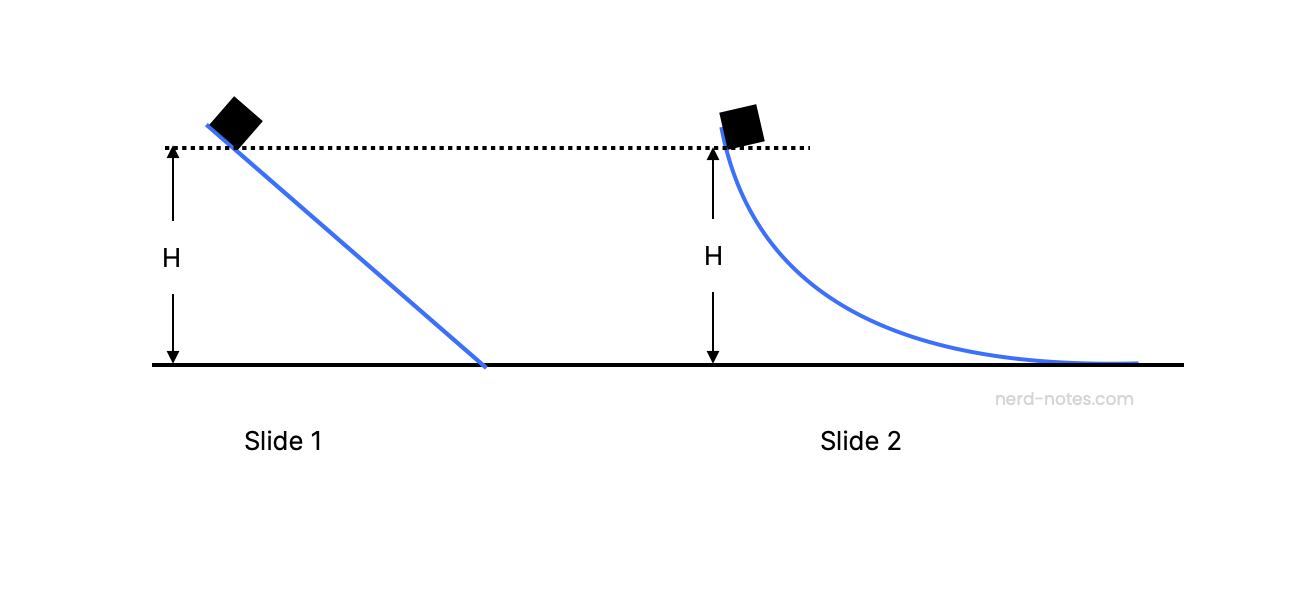 How does the speed \(v_1\) of a block \(m\) reaching the bottom of slide 1 compare with \(v_2\), the speed of a block \(2m\) reaching the end of slide 2? The blocks are released from the same height.
A cardinal (Richmondena cardinalis) of mass \( 3.80 \times 10^{-2} \) \( \text{kg} \) and a baseball of mass \( 0.150 \) \( \text{kg} \) have the same kinetic energy. What is the ratio of the cardinal’s magnitude \( p_c \) of momentum to the magnitude \( p_b \) of the baseball’s momentum?
A man weighing \( 700 \) \( \text{N} \) and a woman weighing \( 400 \) \( \text{N} \) have the same momentum. What is the ratio of the man’s kinetic energy \( K_m \) to that of the woman \( K_w \)?
Two masses \(m_1\) and \(4m_1\) are on an incline. Both surfaces have the same coefficient of kinetic friction. Both objects start from rest at the same height. Which mass has the largest speed at the bottom?
A comet of mass \( m_c = 3.2 \times 10^{14} \) \( \text{kg} \) is orbiting a star with mass \( m_s = 1.8 \times 10^{30} \) \( \text{kg} \). The comet’s orbit is elliptical. At its closest point, the comet is a distance \( r_1 = 8.3 \times 10^{10} \) \( \text{m} \) from the star, and at its farthest point, the comet is a distance \( r_2 = 4.9 \times 10^{11} \) \( \text{m} \) from the star. What is the change in the kinetic energy of the comet as it moves along its orbit from distance \( r_2 \) to distance \( r_1 \) from the star?
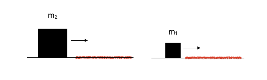
Two blocks, \( m_2 > m_1 \), having the same kinetic energy, move from a frictionless surface onto a surface having friction coefficient \( \mu_k \). Which block will travel further before stopping.
A \( 240 \) \( \text{kg} \) block is dropped from \( 3.0 \) meters onto a spring, compresses the spring and comes to rest.
Two identical arrows, one with \( 2 \) times the speed of the other, are fired into a bale of hay. Assuming the hay exerts a constant “frictional” force on the arrows, the faster arrow will penetrate how much farther than the slower arrow?
On a frictionless horizontal air table, puck A (with mass \( 0.249 \) \( \text{kg} \)) is moving toward puck B (with mass \( 0.375 \) \( \text{kg} \)), which is initially at rest. After the collision, puck A has velocity \( 0.115 \) \( \text{m/s} \) to the left, and puck B has velocity \( 0.645 \) \( \text{m/s} \) to the right.
A \(2 \, \text{kg}\) model rocket is launched with a thrust force of \(275 \, \text{N}\) and reaches a height of \(90 \, \text{m}\), at which point the thrust cuts out, but the rocket continues moving at \(150 \, \text{m/s}\). What is the average air resistance force acting on the rocket during its ascent?
\(\Delta x \approx 5.69\,\text{m}\)
By continuing you (1) agree to our Terms of Use and Terms of Sale and (2) consent to sharing your IP and browser information used by this site’s security protocols as outlined in our Privacy Policy.
| Kinematics | Forces |
|---|---|
| \(\Delta x = v_i t + \frac{1}{2} at^2\) | \(F = ma\) |
| \(v = v_i + at\) | \(F_g = \frac{G m_1 m_2}{r^2}\) |
| \(v^2 = v_i^2 + 2a \Delta x\) | \(f = \mu N\) |
| \(\Delta x = \frac{v_i + v}{2} t\) | \(F_s =-kx\) |
| \(v^2 = v_f^2 \,-\, 2a \Delta x\) |
| Circular Motion | Energy |
|---|---|
| \(F_c = \frac{mv^2}{r}\) | \(KE = \frac{1}{2} mv^2\) |
| \(a_c = \frac{v^2}{r}\) | \(PE = mgh\) |
| \(T = 2\pi \sqrt{\frac{r}{g}}\) | \(KE_i + PE_i = KE_f + PE_f\) |
| \(W = Fd \cos\theta\) |
| Momentum | Torque and Rotations |
|---|---|
| \(p = mv\) | \(\tau = r \cdot F \cdot \sin(\theta)\) |
| \(J = \Delta p\) | \(I = \sum mr^2\) |
| \(p_i = p_f\) | \(L = I \cdot \omega\) |
| Simple Harmonic Motion | Fluids |
|---|---|
| \(F = -kx\) | \(P = \frac{F}{A}\) |
| \(T = 2\pi \sqrt{\frac{l}{g}}\) | \(P_{\text{total}} = P_{\text{atm}} + \rho gh\) |
| \(T = 2\pi \sqrt{\frac{m}{k}}\) | \(Q = Av\) |
| \(x(t) = A \cos(\omega t + \phi)\) | \(F_b = \rho V g\) |
| \(a = -\omega^2 x\) | \(A_1v_1 = A_2v_2\) |
| Constant | Description |
|---|---|
| [katex]g[/katex] | Acceleration due to gravity, typically [katex]9.8 , \text{m/s}^2[/katex] on Earth’s surface |
| [katex]G[/katex] | Universal Gravitational Constant, [katex]6.674 \times 10^{-11} , \text{N} \cdot \text{m}^2/\text{kg}^2[/katex] |
| [katex]\mu_k[/katex] and [katex]\mu_s[/katex] | Coefficients of kinetic ([katex]\mu_k[/katex]) and static ([katex]\mu_s[/katex]) friction, dimensionless. Static friction ([katex]\mu_s[/katex]) is usually greater than kinetic friction ([katex]\mu_k[/katex]) as it resists the start of motion. |
| [katex]k[/katex] | Spring constant, in [katex]\text{N/m}[/katex] |
| [katex] M_E = 5.972 \times 10^{24} , \text{kg} [/katex] | Mass of the Earth |
| [katex] M_M = 7.348 \times 10^{22} , \text{kg} [/katex] | Mass of the Moon |
| [katex] M_M = 1.989 \times 10^{30} , \text{kg} [/katex] | Mass of the Sun |
| Variable | SI Unit |
|---|---|
| [katex]s[/katex] (Displacement) | [katex]\text{meters (m)}[/katex] |
| [katex]v[/katex] (Velocity) | [katex]\text{meters per second (m/s)}[/katex] |
| [katex]a[/katex] (Acceleration) | [katex]\text{meters per second squared (m/s}^2\text{)}[/katex] |
| [katex]t[/katex] (Time) | [katex]\text{seconds (s)}[/katex] |
| [katex]m[/katex] (Mass) | [katex]\text{kilograms (kg)}[/katex] |
| Variable | Derived SI Unit |
|---|---|
| [katex]F[/katex] (Force) | [katex]\text{newtons (N)}[/katex] |
| [katex]E[/katex], [katex]PE[/katex], [katex]KE[/katex] (Energy, Potential Energy, Kinetic Energy) | [katex]\text{joules (J)}[/katex] |
| [katex]P[/katex] (Power) | [katex]\text{watts (W)}[/katex] |
| [katex]p[/katex] (Momentum) | [katex]\text{kilogram meters per second (kgm/s)}[/katex] |
| [katex]\omega[/katex] (Angular Velocity) | [katex]\text{radians per second (rad/s)}[/katex] |
| [katex]\tau[/katex] (Torque) | [katex]\text{newton meters (Nm)}[/katex] |
| [katex]I[/katex] (Moment of Inertia) | [katex]\text{kilogram meter squared (kgm}^2\text{)}[/katex] |
| [katex]f[/katex] (Frequency) | [katex]\text{hertz (Hz)}[/katex] |
Metric Prefixes
Example of using unit analysis: Convert 5 kilometers to millimeters.
Start with the given measurement: [katex]\text{5 km}[/katex]
Use the conversion factors for kilometers to meters and meters to millimeters: [katex]\text{5 km} \times \frac{10^3 \, \text{m}}{1 \, \text{km}} \times \frac{10^3 \, \text{mm}}{1 \, \text{m}}[/katex]
Perform the multiplication: [katex]\text{5 km} \times \frac{10^3 \, \text{m}}{1 \, \text{km}} \times \frac{10^3 \, \text{mm}}{1 \, \text{m}} = 5 \times 10^3 \times 10^3 \, \text{mm}[/katex]
Simplify to get the final answer: [katex]\boxed{5 \times 10^6 \, \text{mm}}[/katex]
Prefix | Symbol | Power of Ten | Equivalent |
|---|---|---|---|
Pico- | p | [katex]10^{-12}[/katex] | 0.000000000001 |
Nano- | n | [katex]10^{-9}[/katex] | 0.000000001 |
Micro- | µ | [katex]10^{-6}[/katex] | 0.000001 |
Milli- | m | [katex]10^{-3}[/katex] | 0.001 |
Centi- | c | [katex]10^{-2}[/katex] | 0.01 |
Deci- | d | [katex]10^{-1}[/katex] | 0.1 |
(Base unit) | – | [katex]10^{0}[/katex] | 1 |
Deca- or Deka- | da | [katex]10^{1}[/katex] | 10 |
Hecto- | h | [katex]10^{2}[/katex] | 100 |
Kilo- | k | [katex]10^{3}[/katex] | 1,000 |
Mega- | M | [katex]10^{6}[/katex] | 1,000,000 |
Giga- | G | [katex]10^{9}[/katex] | 1,000,000,000 |
Tera- | T | [katex]10^{12}[/katex] | 1,000,000,000,000 |
One price to unlock most advanced version of Phy across all our tools.
per month
Billed Monthly. Cancel Anytime.
We crafted THE Ultimate A.P Physics 1 Program so you can learn faster and score higher.
Try our free calculator to see what you need to get a 5 on the 2026 AP Physics 1 exam.
A quick explanation
Credits are used to grade your FRQs and GQs. Pro users get unlimited credits.
Submitting counts as 1 attempt.
Viewing answers or explanations count as a failed attempts.
Phy gives partial credit if needed
MCQs and GQs are are 1 point each. FRQs will state points for each part.
Phy customizes problem explanations based on what you struggle with. Just hit the explanation button to see.
Understand you mistakes quicker.

Phy automatically provides feedback so you can improve your responses.
10 Free Credits To Get You Started

By continuing you agree to nerd-notes.com Terms of Service, Privacy Policy, and our usage of user data.
Feeling uneasy about your next physics test? We'll boost your grade in 3 lessons or less—guaranteed

NEW! PHY AI accurately solves all questions
🔥 Get up to 30% off Elite Physics Tutoring
🧠 NEW! Learn Physics From Scratch Self Paced Course
🎯 Need exam style practice questions?
