| Step | Derivation/Formula | Reasoning |
|---|---|---|
| Analysis of choice (a) | \(x_W = x_{0W} + v_{0W}t + \frac{1}{2}a_Wt^2\) \(x_Z = x_{0Z} + v_{0Z}t + \frac{1}{2}a_Zt^2\) |
(a) uses uniform acceleration equations correctly for each car starting from rest (\(v_{0W} = v_{0Z} = 0\), \(x_{0W}\) and \(x_{0Z}\) are their respective initial positions). Both cars meet when \(x_W = x_Z\). Assuming \(x_{0W}\) is 0 and \(x_{0Z} = d\), solving these equations could indeed yield the time \(t\) when and where they meet. |
| Analysis of choice (b) | \(\Delta x = x – x_0\) | This choice mismanages the given information. The equation for car Z, \(\Delta x = x – x_0\), does not incorporate the acceleration \(a_Z\), thus cannot correctly describe its motion. Moreover, it simplistically assumes constant position change without respect to varying acceleration. |
| Analysis of choice (c) | \(\Delta x = x – x_0\) | Similarly to choice (b), this option for car W does not consider the acceleration \(a_W\). It is also not applicable for a situation where acceleration is not zero, hence inaccurately incorporates the physics of the situation. |
| Analysis of choice (d) | \(\Delta x_W = x – x_0\) and \(\Delta x_Z = x – x_0\) | This choice assumes a fixed displacement for both cars without considering their accelerations, rendering the arrangement ineffective for predicting when and where the cars meet, as it ignores the dynamic nature of the problem. |
| Conclusion | Choice (a) | Only choice (a) correctly applies the physics of uniformly accelerated motion for both cars, allowing for correct prediction of their meeting point. The other choices misrepresent or omit necessary acceleration components. |
A Major Upgrade To Phy Is Coming Soon — Stay Tuned

We'll help clarify entire units in one hour or less — guaranteed.
A self paced course with videos, problems sets, and everything you need to get a 5. Trusted by over 15k students and over 200 schools.
You are standing on a bathroom scale in an elevator. The elevator starts from rest on the first floor and accelerates up to the third floor, \(12 \, \text{m}\) above, in a time of \(6 \, \text{s}\). The scale reads \(800 \, \text{N}\). What is the mass of the person?
A rock is dropped from the top of a tall tower. Half a second later another rock, twice as massive as the first, is dropped. Ignoring air resistance what is the correct choice?
A car moves forward at a steady \( 10 \) \( \text{m/s} \) for \( 5 \) \( \text{s} \). The driver slams the brakes and brings it to rest in \( 2 \) \( \text{s} \). Without waiting, the driver immediately accelerates backward (negative velocity) for \( 3 \) \( \text{s} \) until reaching \( 8 \) \( \text{m/s} \) in reverse. Draw the velocity vs. time graph.
Can an object have \( 0 \) velocity and nonzero acceleration at the same time? Give two examples.
At time \( t = 0 \), a cart is at \( x = 10 \, \text{m} \) and has a velocity of \( 3 \, \text{m/s} \) in the \( -x \) direction. The cart has a constant acceleration in the \( +x \) direction with magnitude \( 3 \, \text{m/s}^2 < a < 6 \, \text{m/s}^2 \). Which of the following gives the possible range of the position of the cart at \( t = 1 \, \text{s} \)?
A car travels at \( 20 \, \text{m/s} \) for \( 5 \, \text{mins} \) and then travels another \( 2 \, \text{km} \) at \( 40 \, \text{m/s} \). What is the total distance traveled and time of travel for the car?
A car is driving at \(25 \, \text{m/s}\) when a light turns red \(100 \, \text{m}\) ahead. The driver takes an unknown amount of time to react and hit the brakes, but manages to skid to a stop at the red light. If \(\mu_s = 0.9\) and \(\mu_k = 0.65\), what was the reaction time of the driver?
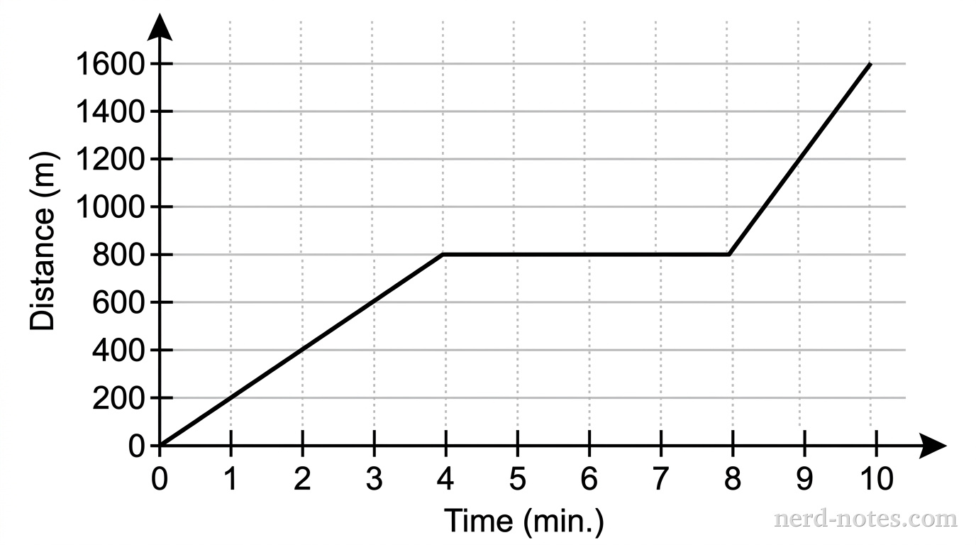
On Saturday, Ashley rode her bicycle to visit Maria. Maria’s house is directly east of Ashley’s. The graph shows how far Ashley was from her house after each minute of her trip. (Hint – Use the standard units of velocity \(\text{m/s}\) for all parts)
A coin is dropped from a hot air-balloon that is \(250 \, \text{m}\) above the ground rising at \(11 \, \text{m/s}\) upwards. For the coin, assume up is positive and find the following:
A driver is traveling at a speed of \( 18.0 \) \( \text{m/s} \) when she sees a red light ahead. Her car is capable of decelerating at a rate of \( 3.65 \) \( \text{m/s}^2 \). If it takes her \( 0.350 \) \( \text{s} \) to get the brakes on and she is \( 20.0 \) \( \text{m} \) from the intersection when she sees the light, will she be able to stop in time? How far from the beginning of the intersection will she be, and in what direction?
By continuing you (1) agree to our Terms of Use and Terms of Sale and (2) consent to sharing your IP and browser information used by this site’s security protocols as outlined in our Privacy Policy.
| Kinematics | Forces |
|---|---|
| \(\Delta x = v_i t + \frac{1}{2} at^2\) | \(F = ma\) |
| \(v = v_i + at\) | \(F_g = \frac{G m_1 m_2}{r^2}\) |
| \(v^2 = v_i^2 + 2a \Delta x\) | \(f = \mu N\) |
| \(\Delta x = \frac{v_i + v}{2} t\) | \(F_s =-kx\) |
| \(v^2 = v_f^2 \,-\, 2a \Delta x\) |
| Circular Motion | Energy |
|---|---|
| \(F_c = \frac{mv^2}{r}\) | \(KE = \frac{1}{2} mv^2\) |
| \(a_c = \frac{v^2}{r}\) | \(PE = mgh\) |
| \(T = 2\pi \sqrt{\frac{r}{g}}\) | \(KE_i + PE_i = KE_f + PE_f\) |
| \(W = Fd \cos\theta\) |
| Momentum | Torque and Rotations |
|---|---|
| \(p = mv\) | \(\tau = r \cdot F \cdot \sin(\theta)\) |
| \(J = \Delta p\) | \(I = \sum mr^2\) |
| \(p_i = p_f\) | \(L = I \cdot \omega\) |
| Simple Harmonic Motion | Fluids |
|---|---|
| \(F = -kx\) | \(P = \frac{F}{A}\) |
| \(T = 2\pi \sqrt{\frac{l}{g}}\) | \(P_{\text{total}} = P_{\text{atm}} + \rho gh\) |
| \(T = 2\pi \sqrt{\frac{m}{k}}\) | \(Q = Av\) |
| \(x(t) = A \cos(\omega t + \phi)\) | \(F_b = \rho V g\) |
| \(a = -\omega^2 x\) | \(A_1v_1 = A_2v_2\) |
| Constant | Description |
|---|---|
| [katex]g[/katex] | Acceleration due to gravity, typically [katex]9.8 , \text{m/s}^2[/katex] on Earth’s surface |
| [katex]G[/katex] | Universal Gravitational Constant, [katex]6.674 \times 10^{-11} , \text{N} \cdot \text{m}^2/\text{kg}^2[/katex] |
| [katex]\mu_k[/katex] and [katex]\mu_s[/katex] | Coefficients of kinetic ([katex]\mu_k[/katex]) and static ([katex]\mu_s[/katex]) friction, dimensionless. Static friction ([katex]\mu_s[/katex]) is usually greater than kinetic friction ([katex]\mu_k[/katex]) as it resists the start of motion. |
| [katex]k[/katex] | Spring constant, in [katex]\text{N/m}[/katex] |
| [katex] M_E = 5.972 \times 10^{24} , \text{kg} [/katex] | Mass of the Earth |
| [katex] M_M = 7.348 \times 10^{22} , \text{kg} [/katex] | Mass of the Moon |
| [katex] M_M = 1.989 \times 10^{30} , \text{kg} [/katex] | Mass of the Sun |
| Variable | SI Unit |
|---|---|
| [katex]s[/katex] (Displacement) | [katex]\text{meters (m)}[/katex] |
| [katex]v[/katex] (Velocity) | [katex]\text{meters per second (m/s)}[/katex] |
| [katex]a[/katex] (Acceleration) | [katex]\text{meters per second squared (m/s}^2\text{)}[/katex] |
| [katex]t[/katex] (Time) | [katex]\text{seconds (s)}[/katex] |
| [katex]m[/katex] (Mass) | [katex]\text{kilograms (kg)}[/katex] |
| Variable | Derived SI Unit |
|---|---|
| [katex]F[/katex] (Force) | [katex]\text{newtons (N)}[/katex] |
| [katex]E[/katex], [katex]PE[/katex], [katex]KE[/katex] (Energy, Potential Energy, Kinetic Energy) | [katex]\text{joules (J)}[/katex] |
| [katex]P[/katex] (Power) | [katex]\text{watts (W)}[/katex] |
| [katex]p[/katex] (Momentum) | [katex]\text{kilogram meters per second (kgm/s)}[/katex] |
| [katex]\omega[/katex] (Angular Velocity) | [katex]\text{radians per second (rad/s)}[/katex] |
| [katex]\tau[/katex] (Torque) | [katex]\text{newton meters (Nm)}[/katex] |
| [katex]I[/katex] (Moment of Inertia) | [katex]\text{kilogram meter squared (kgm}^2\text{)}[/katex] |
| [katex]f[/katex] (Frequency) | [katex]\text{hertz (Hz)}[/katex] |
Metric Prefixes
Example of using unit analysis: Convert 5 kilometers to millimeters.
Start with the given measurement: [katex]\text{5 km}[/katex]
Use the conversion factors for kilometers to meters and meters to millimeters: [katex]\text{5 km} \times \frac{10^3 \, \text{m}}{1 \, \text{km}} \times \frac{10^3 \, \text{mm}}{1 \, \text{m}}[/katex]
Perform the multiplication: [katex]\text{5 km} \times \frac{10^3 \, \text{m}}{1 \, \text{km}} \times \frac{10^3 \, \text{mm}}{1 \, \text{m}} = 5 \times 10^3 \times 10^3 \, \text{mm}[/katex]
Simplify to get the final answer: [katex]\boxed{5 \times 10^6 \, \text{mm}}[/katex]
Prefix | Symbol | Power of Ten | Equivalent |
|---|---|---|---|
Pico- | p | [katex]10^{-12}[/katex] | 0.000000000001 |
Nano- | n | [katex]10^{-9}[/katex] | 0.000000001 |
Micro- | µ | [katex]10^{-6}[/katex] | 0.000001 |
Milli- | m | [katex]10^{-3}[/katex] | 0.001 |
Centi- | c | [katex]10^{-2}[/katex] | 0.01 |
Deci- | d | [katex]10^{-1}[/katex] | 0.1 |
(Base unit) | – | [katex]10^{0}[/katex] | 1 |
Deca- or Deka- | da | [katex]10^{1}[/katex] | 10 |
Hecto- | h | [katex]10^{2}[/katex] | 100 |
Kilo- | k | [katex]10^{3}[/katex] | 1,000 |
Mega- | M | [katex]10^{6}[/katex] | 1,000,000 |
Giga- | G | [katex]10^{9}[/katex] | 1,000,000,000 |
Tera- | T | [katex]10^{12}[/katex] | 1,000,000,000,000 |
One price to unlock most advanced version of Phy across all our tools.
per month
Billed Monthly. Cancel Anytime.
We crafted THE Ultimate A.P Physics 1 Program so you can learn faster and score higher.
Try our free calculator to see what you need to get a 5 on the 2026 AP Physics 1 exam.
A quick explanation
Credits are used to grade your FRQs and GQs. Pro users get unlimited credits.
Submitting counts as 1 attempt.
Viewing answers or explanations count as a failed attempts.
Phy gives partial credit if needed
MCQs and GQs are are 1 point each. FRQs will state points for each part.
Phy customizes problem explanations based on what you struggle with. Just hit the explanation button to see.
Understand you mistakes quicker.

Phy automatically provides feedback so you can improve your responses.
10 Free Credits To Get You Started

By continuing you agree to nerd-notes.com Terms of Service, Privacy Policy, and our usage of user data.
Feeling uneasy about your next physics test? We'll boost your grade in 3 lessons or less—guaranteed

NEW! PHY AI accurately solves all questions
🔥 Get up to 30% off Elite Physics Tutoring
🧠 NEW! Learn Physics From Scratch Self Paced Course
🎯 Need exam style practice questions?
