| Step | Derivation/Formula | Reasoning |
|---|---|---|
| Analysis of choice (a) | \(x_W = x_{0W} + v_{0W}t + \frac{1}{2}a_Wt^2\) \(x_Z = x_{0Z} + v_{0Z}t + \frac{1}{2}a_Zt^2\) |
(a) uses uniform acceleration equations correctly for each car starting from rest (\(v_{0W} = v_{0Z} = 0\), \(x_{0W}\) and \(x_{0Z}\) are their respective initial positions). Both cars meet when \(x_W = x_Z\). Assuming \(x_{0W}\) is 0 and \(x_{0Z} = d\), solving these equations could indeed yield the time \(t\) when and where they meet. |
| Analysis of choice (b) | \(\Delta x = x – x_0\) | This choice mismanages the given information. The equation for car Z, \(\Delta x = x – x_0\), does not incorporate the acceleration \(a_Z\), thus cannot correctly describe its motion. Moreover, it simplistically assumes constant position change without respect to varying acceleration. |
| Analysis of choice (c) | \(\Delta x = x – x_0\) | Similarly to choice (b), this option for car W does not consider the acceleration \(a_W\). It is also not applicable for a situation where acceleration is not zero, hence inaccurately incorporates the physics of the situation. |
| Analysis of choice (d) | \(\Delta x_W = x – x_0\) and \(\Delta x_Z = x – x_0\) | This choice assumes a fixed displacement for both cars without considering their accelerations, rendering the arrangement ineffective for predicting when and where the cars meet, as it ignores the dynamic nature of the problem. |
| Conclusion | Choice (a) | Only choice (a) correctly applies the physics of uniformly accelerated motion for both cars, allowing for correct prediction of their meeting point. The other choices misrepresent or omit necessary acceleration components. |
A Major Upgrade To Phy Is Coming Soon — Stay Tuned

We'll help clarify entire units in one hour or less — guaranteed.
A self paced course with videos, problems sets, and everything you need to get a 5. Trusted by over 15k students and over 200 schools.
Two balls are dropped off a cliff, 3 seconds apart. The first ball dropped is twice as heavy as the second ball dropped. Air resistance is negligible. While both balls are falling, the distance between the two balls is
Ball 1 is dropped from rest at time \( t = 0 \) from a tower of height \( h \). At the same instant, ball 2 is launched upward from the ground with the initial speed \( v_0 \). If air resistance is negligible, at what time \( t \) will the two balls pass each other?
An ice sled powered by a rocket engine starts from rest on a large frozen lake and accelerates at \( +13.0 \, \text{m/s}^2 \). At \( t_1 \), the rocket engine is shut down and the sled moves with constant velocity \( v \) until \( t_2 \). The total distance traveled by the sled is \( 5.30 \times 10^3 \, \text{m} \) and the total time is \( 90.0 \, \text{s} \).
Which of these scenarios involve accelerated motion? (Select all that apply)
A stone is thrown vertically upward with a speed of \( 24.0 \) \( \text{m/s} \).
A car accelerates from rest with an acceleration of \( 4.3 \, \text{m/s}^2 \) for a time of \( 6.8 \, \text{s} \). The car then slows to a stop with an acceleration of \( 5.1 \, \text{m/s}^2 \). What is the total distance traveled by the car?
A ball is launched horizontally from a height. At the same time, another ball is dropped vertically from the same height. Which hits the ground first?
Mary and Sally are in a foot race. When Mary is \( 22 \) \( \text{m} \) from the finish line, she has a speed of \( 4.0 \) \( \text{m/s} \) and is \( 5.0 \) \( \text{m} \) behind Sally, who has a speed of \( 5.0 \) \( \text{m/s} \). Sally thinks she has an easy win and, during the remaining portion of the race, decelerates at a constant rate of \( 0.40 \) \( \text{m/s}^2 \) until she reaches the finish line. What constant acceleration must Mary maintain during the remaining portion of the race if she wishes to cross the finish line side-by-side with Sally?
By continuing you (1) agree to our Terms of Use and Terms of Sale and (2) consent to sharing your IP and browser information used by this site’s security protocols as outlined in our Privacy Policy.
| Kinematics | Forces |
|---|---|
| \(\Delta x = v_i t + \frac{1}{2} at^2\) | \(F = ma\) |
| \(v = v_i + at\) | \(F_g = \frac{G m_1 m_2}{r^2}\) |
| \(v^2 = v_i^2 + 2a \Delta x\) | \(f = \mu N\) |
| \(\Delta x = \frac{v_i + v}{2} t\) | \(F_s =-kx\) |
| \(v^2 = v_f^2 \,-\, 2a \Delta x\) |
| Circular Motion | Energy |
|---|---|
| \(F_c = \frac{mv^2}{r}\) | \(KE = \frac{1}{2} mv^2\) |
| \(a_c = \frac{v^2}{r}\) | \(PE = mgh\) |
| \(T = 2\pi \sqrt{\frac{r}{g}}\) | \(KE_i + PE_i = KE_f + PE_f\) |
| \(W = Fd \cos\theta\) |
| Momentum | Torque and Rotations |
|---|---|
| \(p = mv\) | \(\tau = r \cdot F \cdot \sin(\theta)\) |
| \(J = \Delta p\) | \(I = \sum mr^2\) |
| \(p_i = p_f\) | \(L = I \cdot \omega\) |
| Simple Harmonic Motion | Fluids |
|---|---|
| \(F = -kx\) | \(P = \frac{F}{A}\) |
| \(T = 2\pi \sqrt{\frac{l}{g}}\) | \(P_{\text{total}} = P_{\text{atm}} + \rho gh\) |
| \(T = 2\pi \sqrt{\frac{m}{k}}\) | \(Q = Av\) |
| \(x(t) = A \cos(\omega t + \phi)\) | \(F_b = \rho V g\) |
| \(a = -\omega^2 x\) | \(A_1v_1 = A_2v_2\) |
| Constant | Description |
|---|---|
| [katex]g[/katex] | Acceleration due to gravity, typically [katex]9.8 , \text{m/s}^2[/katex] on Earth’s surface |
| [katex]G[/katex] | Universal Gravitational Constant, [katex]6.674 \times 10^{-11} , \text{N} \cdot \text{m}^2/\text{kg}^2[/katex] |
| [katex]\mu_k[/katex] and [katex]\mu_s[/katex] | Coefficients of kinetic ([katex]\mu_k[/katex]) and static ([katex]\mu_s[/katex]) friction, dimensionless. Static friction ([katex]\mu_s[/katex]) is usually greater than kinetic friction ([katex]\mu_k[/katex]) as it resists the start of motion. |
| [katex]k[/katex] | Spring constant, in [katex]\text{N/m}[/katex] |
| [katex] M_E = 5.972 \times 10^{24} , \text{kg} [/katex] | Mass of the Earth |
| [katex] M_M = 7.348 \times 10^{22} , \text{kg} [/katex] | Mass of the Moon |
| [katex] M_M = 1.989 \times 10^{30} , \text{kg} [/katex] | Mass of the Sun |
| Variable | SI Unit |
|---|---|
| [katex]s[/katex] (Displacement) | [katex]\text{meters (m)}[/katex] |
| [katex]v[/katex] (Velocity) | [katex]\text{meters per second (m/s)}[/katex] |
| [katex]a[/katex] (Acceleration) | [katex]\text{meters per second squared (m/s}^2\text{)}[/katex] |
| [katex]t[/katex] (Time) | [katex]\text{seconds (s)}[/katex] |
| [katex]m[/katex] (Mass) | [katex]\text{kilograms (kg)}[/katex] |
| Variable | Derived SI Unit |
|---|---|
| [katex]F[/katex] (Force) | [katex]\text{newtons (N)}[/katex] |
| [katex]E[/katex], [katex]PE[/katex], [katex]KE[/katex] (Energy, Potential Energy, Kinetic Energy) | [katex]\text{joules (J)}[/katex] |
| [katex]P[/katex] (Power) | [katex]\text{watts (W)}[/katex] |
| [katex]p[/katex] (Momentum) | [katex]\text{kilogram meters per second (kgm/s)}[/katex] |
| [katex]\omega[/katex] (Angular Velocity) | [katex]\text{radians per second (rad/s)}[/katex] |
| [katex]\tau[/katex] (Torque) | [katex]\text{newton meters (Nm)}[/katex] |
| [katex]I[/katex] (Moment of Inertia) | [katex]\text{kilogram meter squared (kgm}^2\text{)}[/katex] |
| [katex]f[/katex] (Frequency) | [katex]\text{hertz (Hz)}[/katex] |
Metric Prefixes
Example of using unit analysis: Convert 5 kilometers to millimeters.
Start with the given measurement: [katex]\text{5 km}[/katex]
Use the conversion factors for kilometers to meters and meters to millimeters: [katex]\text{5 km} \times \frac{10^3 \, \text{m}}{1 \, \text{km}} \times \frac{10^3 \, \text{mm}}{1 \, \text{m}}[/katex]
Perform the multiplication: [katex]\text{5 km} \times \frac{10^3 \, \text{m}}{1 \, \text{km}} \times \frac{10^3 \, \text{mm}}{1 \, \text{m}} = 5 \times 10^3 \times 10^3 \, \text{mm}[/katex]
Simplify to get the final answer: [katex]\boxed{5 \times 10^6 \, \text{mm}}[/katex]
Prefix | Symbol | Power of Ten | Equivalent |
|---|---|---|---|
Pico- | p | [katex]10^{-12}[/katex] | 0.000000000001 |
Nano- | n | [katex]10^{-9}[/katex] | 0.000000001 |
Micro- | µ | [katex]10^{-6}[/katex] | 0.000001 |
Milli- | m | [katex]10^{-3}[/katex] | 0.001 |
Centi- | c | [katex]10^{-2}[/katex] | 0.01 |
Deci- | d | [katex]10^{-1}[/katex] | 0.1 |
(Base unit) | – | [katex]10^{0}[/katex] | 1 |
Deca- or Deka- | da | [katex]10^{1}[/katex] | 10 |
Hecto- | h | [katex]10^{2}[/katex] | 100 |
Kilo- | k | [katex]10^{3}[/katex] | 1,000 |
Mega- | M | [katex]10^{6}[/katex] | 1,000,000 |
Giga- | G | [katex]10^{9}[/katex] | 1,000,000,000 |
Tera- | T | [katex]10^{12}[/katex] | 1,000,000,000,000 |
One price to unlock most advanced version of Phy across all our tools.
per month
Billed Monthly. Cancel Anytime.
Try our free calculator to see what you need to get a 5 on the 2026 AP Physics 1 exam.
A quick explanation
Credits are used to grade your FRQs and GQs. Pro users get unlimited credits.
Submitting counts as 1 attempt.
Viewing answers or explanations count as a failed attempts.
Phy gives partial credit if needed
MCQs and GQs are are 1 point each. FRQs will state points for each part.
Phy customizes problem explanations based on what you struggle with. Just hit the explanation button to see.
Understand you mistakes quicker.

Phy automatically provides feedback so you can improve your responses.
10 Free Credits To Get You Started

By continuing you agree to nerd-notes.com Terms of Service, Privacy Policy, and our usage of user data.
Feeling uneasy about your next physics test? We'll boost your grade in 3 lessons or less—guaranteed

NEW! PHY AI accurately solves all questions
🔥 Get up to 30% off Elite Physics Tutoring
🧠 NEW! Learn Physics From Scratch Self Paced Course
🎯 Need exam style practice questions?
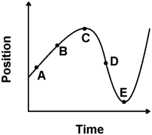 Based on this graph…