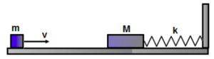
A small block moving with a constant speed \(v\) collides inelastically with a block \(M\) attached to one end of a spring \(k\). The other end of the spring is connected to a stationary wall. Ignore friction between the blocks and the surface.
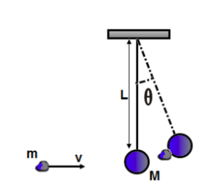
A \(20 \, \text{g}\) piece of clay moving at a speed of \(50 \, \text{m/s}\) strikes a \(500 \, \text{g}\) pendulum bob at rest. The length of a string is \(0.8 \, \text{m}\). After the collision, the clay-bob system starts to oscillate as a simple pendulum.

A block of mass \( 0.5 \) \( \text{kg} \) is attached to a horizontal spring with a spring constant of \( 150 \) \( \text{N/m} \). The block is released from rest at position \( x = 0.05 \) \( \text{m} \), as shown, and undergoes simple harmonic motion, reaching a maximum position of \( x = 0.1 \) \( \text{m} \). The speed of the block when it passes through position \( x = 0.09 \) \( \text{m} \) is most nearly
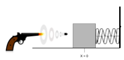
A bullet (mass: \(0.05 \, \text{kg}\)) is fired horizontally (\(v = 200 \, \text{m/s}\)) at a block (mass: \(1.3 \, \text{kg}\)) initially at rest on a frictionless surface. The block is attached to a spring (\(k = 2500 \, \text{N/m}\)). The bullet becomes embedded. Calculate:

A block is attached to a horizontal spring and is initially at rest at the equilibrium position \( x = 0 \), as shown in Figure \( 1 \). The block is then moved to position \( x = -A \), as shown in Figure \( 2 \), and released from rest, undergoing simple harmonic motion. At the instant the block reaches position \( x = +A \), another identical block is dropped onto and sticks to the block, as shown in Figure \( 3 \). The two–block–spring system then continues to undergo simple harmonic motion. Which of the following correctly compares the total mechanical energy \( E_{\text{tot},2} \) of the two–block–spring system after the collision to the total mechanical energy \( E_{\text{tot},1} \) of the one–block–spring system before the collision?


