| Derivation/Formula | Reasoning |
|---|---|
| \[\Delta x_1 = \frac{1}{2} a_1 t_1^2\] | For motion starting from rest under constant acceleration, the displacement is \( \Delta x = \frac{1}{2} a t^2 \). |
| \[\Delta x_1 = \frac{1}{2} (4.3)(6.8)^2 = 99.4\,\text{m}\] | Substitute \( a_1 = 4.3\,\text{m/s}^2 \) and \( t_1 = 6.8\,\text{s} \) to obtain the distance covered while speeding up. |
| \[v_x = a_1 t_1\] | The final speed after the first interval is given by \( v = a t \) since \( v_i = 0 \). |
| \[v_x = (4.3)(6.8) = 29.24\,\text{m/s}\] | Insert the known values to compute the speed just before braking. |
| \[\Delta x_2 = \frac{v_x^2}{2 a_2}\] | Re-arrange \( 0 = v_x^2 + 2(-a_2)\Delta x_2 \) to find the stopping distance with constant deceleration \( a_2 \). |
| \[\Delta x_2 = \frac{(29.24)^2}{2(5.1)} = 83.8\,\text{m}\] | Plug in \( v_x = 29.24\,\text{m/s} \) and \( a_2 = 5.1\,\text{m/s}^2 \). |
| \[\Delta x_{\text{total}} = \Delta x_1 + \Delta x_2\] | Total distance is the sum of the distances during acceleration and deceleration. |
| \[\Delta x_{\text{total}} = 99.4\,\text{m} + 83.8\,\text{m} = 183\,\text{m}\] | Add the two segments to obtain the total displacement. |
A Major Upgrade To Phy Is Coming Soon — Stay Tuned
We'll help clarify entire units in one hour or less — guaranteed.
A car moving at 30 m/s makes a head-on collision with a stone wall. From what height would the car have to fall in order to make an equally hard collision with the ground?
A baseball is tossed from street level by a student straight up at a speed of \(25.3 \text{ m/s}\). After reaching maximum height, it is caught by another student on the roof of a building, \(17.4 \text{ m}\) above the street. How long did this take?
A cart starts from rest and accelerates uniformly at 4.0 m/s2 for 5.0 s. It next maintains the velocity it has reached for 10 s. Then it slows down at a steady rate of 2.0 m/s2 for 4.0 s. What is the final speed of the car?
A body moving in the positive \( x \) direction passes the origin at time \( t = 0 \). Between \( t = 0 \) and \( t = 1 \, \text{second} \), the body has a constant speed of \( 24 \, \text{m/s} \). At \( t = 1 \, \text{second} \), the body is given a constant acceleration of \( 6 \, \text{m/s}^2 \) in the negative \( x \) direction. The position \( x \) of the body at \( t = 11 \, \text{seconds} \) is
A 135.0 N force is applied to a 30.0 kg box at 42 degree angle to the horizontal. If the force of friction is 85.0, what is the net force and acceleration? If the object starts from rest, how far has it traveled in 3.3 sec?
An elevator of height \(h\) ascends with constant acceleration \(a\). When it crosses a platform, it has acquired a velocity \(u\). At this instant a bolt drops from the top of the elevator. Find the time for the bolt to hit the floor of the elevator. Give your answer in terms of \(h\), \(a\), and any constant.
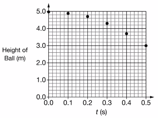
On another planet, a ball is in free fall after being released from rest at time \( t = 0 \). A graph of the height of the ball above the planet’s surface as a function of time \( t \) is shown. The acceleration due to gravity on the planet is most nearly
A student is running at her top speed of \( 5.0 \, \text{m/s} \) to catch a bus, which is stopped at the bus stop. When the student is still \( 40.0 \, \text{m} \) from the bus, it starts to pull away, moving with a constant acceleration of \( 0.170 \, \text{m/s}^2 \).
You drive \( 4 \) \( \text{km} \) at \( 30 \) \( \text{km/h} \) and then another \( 4 \) \( \text{km} \) at \( 50 \) \( \text{km/h} \). What is your average speed for the whole \( 8 \) \( \text{km} \) trip?
A projectile of mass 0.750 kg is shot straight up with an initial speed of 18.0 m/s.
\(183\,\text{m}\)
By continuing you (1) agree to our Terms of Use and Terms of Sale and (2) consent to sharing your IP and browser information used by this site’s security protocols as outlined in our Privacy Policy.
| Kinematics | Forces |
|---|---|
| \(\Delta x = v_i t + \frac{1}{2} at^2\) | \(F = ma\) |
| \(v = v_i + at\) | \(F_g = \frac{G m_1 m_2}{r^2}\) |
| \(v^2 = v_i^2 + 2a \Delta x\) | \(f = \mu N\) |
| \(\Delta x = \frac{v_i + v}{2} t\) | \(F_s =-kx\) |
| \(v^2 = v_f^2 \,-\, 2a \Delta x\) |
| Circular Motion | Energy |
|---|---|
| \(F_c = \frac{mv^2}{r}\) | \(KE = \frac{1}{2} mv^2\) |
| \(a_c = \frac{v^2}{r}\) | \(PE = mgh\) |
| \(T = 2\pi \sqrt{\frac{r}{g}}\) | \(KE_i + PE_i = KE_f + PE_f\) |
| \(W = Fd \cos\theta\) |
| Momentum | Torque and Rotations |
|---|---|
| \(p = mv\) | \(\tau = r \cdot F \cdot \sin(\theta)\) |
| \(J = \Delta p\) | \(I = \sum mr^2\) |
| \(p_i = p_f\) | \(L = I \cdot \omega\) |
| Simple Harmonic Motion | Fluids |
|---|---|
| \(F = -kx\) | \(P = \frac{F}{A}\) |
| \(T = 2\pi \sqrt{\frac{l}{g}}\) | \(P_{\text{total}} = P_{\text{atm}} + \rho gh\) |
| \(T = 2\pi \sqrt{\frac{m}{k}}\) | \(Q = Av\) |
| \(x(t) = A \cos(\omega t + \phi)\) | \(F_b = \rho V g\) |
| \(a = -\omega^2 x\) | \(A_1v_1 = A_2v_2\) |
| Constant | Description |
|---|---|
| [katex]g[/katex] | Acceleration due to gravity, typically [katex]9.8 , \text{m/s}^2[/katex] on Earth’s surface |
| [katex]G[/katex] | Universal Gravitational Constant, [katex]6.674 \times 10^{-11} , \text{N} \cdot \text{m}^2/\text{kg}^2[/katex] |
| [katex]\mu_k[/katex] and [katex]\mu_s[/katex] | Coefficients of kinetic ([katex]\mu_k[/katex]) and static ([katex]\mu_s[/katex]) friction, dimensionless. Static friction ([katex]\mu_s[/katex]) is usually greater than kinetic friction ([katex]\mu_k[/katex]) as it resists the start of motion. |
| [katex]k[/katex] | Spring constant, in [katex]\text{N/m}[/katex] |
| [katex] M_E = 5.972 \times 10^{24} , \text{kg} [/katex] | Mass of the Earth |
| [katex] M_M = 7.348 \times 10^{22} , \text{kg} [/katex] | Mass of the Moon |
| [katex] M_M = 1.989 \times 10^{30} , \text{kg} [/katex] | Mass of the Sun |
| Variable | SI Unit |
|---|---|
| [katex]s[/katex] (Displacement) | [katex]\text{meters (m)}[/katex] |
| [katex]v[/katex] (Velocity) | [katex]\text{meters per second (m/s)}[/katex] |
| [katex]a[/katex] (Acceleration) | [katex]\text{meters per second squared (m/s}^2\text{)}[/katex] |
| [katex]t[/katex] (Time) | [katex]\text{seconds (s)}[/katex] |
| [katex]m[/katex] (Mass) | [katex]\text{kilograms (kg)}[/katex] |
| Variable | Derived SI Unit |
|---|---|
| [katex]F[/katex] (Force) | [katex]\text{newtons (N)}[/katex] |
| [katex]E[/katex], [katex]PE[/katex], [katex]KE[/katex] (Energy, Potential Energy, Kinetic Energy) | [katex]\text{joules (J)}[/katex] |
| [katex]P[/katex] (Power) | [katex]\text{watts (W)}[/katex] |
| [katex]p[/katex] (Momentum) | [katex]\text{kilogram meters per second (kgm/s)}[/katex] |
| [katex]\omega[/katex] (Angular Velocity) | [katex]\text{radians per second (rad/s)}[/katex] |
| [katex]\tau[/katex] (Torque) | [katex]\text{newton meters (Nm)}[/katex] |
| [katex]I[/katex] (Moment of Inertia) | [katex]\text{kilogram meter squared (kgm}^2\text{)}[/katex] |
| [katex]f[/katex] (Frequency) | [katex]\text{hertz (Hz)}[/katex] |
Metric Prefixes
Example of using unit analysis: Convert 5 kilometers to millimeters.
Start with the given measurement: [katex]\text{5 km}[/katex]
Use the conversion factors for kilometers to meters and meters to millimeters: [katex]\text{5 km} \times \frac{10^3 \, \text{m}}{1 \, \text{km}} \times \frac{10^3 \, \text{mm}}{1 \, \text{m}}[/katex]
Perform the multiplication: [katex]\text{5 km} \times \frac{10^3 \, \text{m}}{1 \, \text{km}} \times \frac{10^3 \, \text{mm}}{1 \, \text{m}} = 5 \times 10^3 \times 10^3 \, \text{mm}[/katex]
Simplify to get the final answer: [katex]\boxed{5 \times 10^6 \, \text{mm}}[/katex]
Prefix | Symbol | Power of Ten | Equivalent |
|---|---|---|---|
Pico- | p | [katex]10^{-12}[/katex] | 0.000000000001 |
Nano- | n | [katex]10^{-9}[/katex] | 0.000000001 |
Micro- | µ | [katex]10^{-6}[/katex] | 0.000001 |
Milli- | m | [katex]10^{-3}[/katex] | 0.001 |
Centi- | c | [katex]10^{-2}[/katex] | 0.01 |
Deci- | d | [katex]10^{-1}[/katex] | 0.1 |
(Base unit) | – | [katex]10^{0}[/katex] | 1 |
Deca- or Deka- | da | [katex]10^{1}[/katex] | 10 |
Hecto- | h | [katex]10^{2}[/katex] | 100 |
Kilo- | k | [katex]10^{3}[/katex] | 1,000 |
Mega- | M | [katex]10^{6}[/katex] | 1,000,000 |
Giga- | G | [katex]10^{9}[/katex] | 1,000,000,000 |
Tera- | T | [katex]10^{12}[/katex] | 1,000,000,000,000 |
One price to unlock most advanced version of Phy across all our tools.
per month
Billed Monthly. Cancel Anytime.
We crafted THE Ultimate A.P Physics 1 Program so you can learn faster and score higher.
Try our free calculator to see what you need to get a 5 on the 2026 AP Physics 1 exam.
A quick explanation
Credits are used to grade your FRQs and GQs. Pro users get unlimited credits.
Submitting counts as 1 attempt.
Viewing answers or explanations count as a failed attempts.
Phy gives partial credit if needed
MCQs and GQs are are 1 point each. FRQs will state points for each part.
Phy customizes problem explanations based on what you struggle with. Just hit the explanation button to see.
Understand you mistakes quicker.

Phy automatically provides feedback so you can improve your responses.
10 Free Credits To Get You Started

By continuing you agree to nerd-notes.com Terms of Service, Privacy Policy, and our usage of user data.
Feeling uneasy about your next physics test? We'll boost your grade in 3 lessons or less—guaranteed

NEW! PHY AI accurately solves all questions
🔥 Get up to 30% off Elite Physics Tutoring
🧠 NEW! Learn Physics From Scratch Self Paced Course
🎯 Need exam style practice questions?
