| Step | Derivation/Formula | Reasoning |
|---|---|---|
| (a) How much time does it take for a diver to reach the water? | ||
| 1 | Use the vertical motion equation:
\( y = y_0 + v_{0y} t + \dfrac{1}{2} a t^2 \) |
Relates vertical position, initial velocity, time, and acceleration. |
| 2 | Set final position \( y = 0 \, \text{m} \), initial position \( y_0 = 36 \, \text{m} \), initial velocity \( v_{0y} = +2 \, \text{m/s} \), and acceleration \( a = -9.8 \, \text{m/s}^2 \):
\( 0 = 36 + 2 t – 4.9 t^2 \) |
Plugged in known values; acceleration is negative due to gravity. |
| 3 | Rearrange the equation to standard quadratic form:
\( -4.9 t^2 + 2 t + 36 = 0 \) |
Prepared to solve the quadratic equation for \( t \). |
| 4 | Use the quadratic formula \( t = \dfrac{-b \pm \sqrt{b^2 – 4ac}}{2a} \), where \( a = 4.9 \), \( b = -2 \), \( c = -36 \):
Discriminant \( D = b^2 – 4ac \): |
Calculated the discriminant for the quadratic equation. |
| 5 | Solve for \( t \):
\( t = \dfrac{-b \pm \sqrt{D}}{2a} = \dfrac{-(-2) \pm \sqrt{709.6}}{2 \times 4.9} \) |
Applied quadratic formula to find possible values of \( t \). |
| 6 | Select the positive root (physical solution):
\( t = \dfrac{2 + 26.65}{9.8} \approx \dfrac{28.65}{9.8} \approx 2.92 \, \text{s} \) |
Negative time is not physically meaningful here; chose positive time. |
| (b) What is the diver’s velocity right before they hit the water? | ||
| 7 | Use the velocity equation:
\( v = v_0 + a t \) |
Relates final velocity, initial velocity, acceleration, and time. |
| 8 | Substitute known values \( v_0 = +2 \, \text{m/s} \), \( a = -9.8 \, \text{m/s}^2 \), \( t = 2.92 \, \text{s} \):
\( v = 2 + (-9.8)(2.92) \) |
Calculated final velocity; negative sign indicates downward direction. |
| 9 | Express the speed and direction:
The diver’s speed is \( 26.62 \, \text{m/s} \) downward. |
Provided the magnitude and clarified the direction. |
A Major Upgrade To Phy Is Coming Soon — Stay Tuned

We'll help clarify entire units in one hour or less — guaranteed.
A self paced course with videos, problems sets, and everything you need to get a 5. Trusted by over 15k students and over 200 schools.
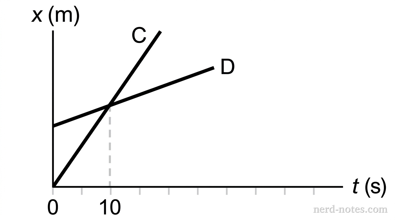
The figure shows a graph of the position \(x\) of two cars, \(C\) and \(D\), as a function of time \(t\). According to this graph, which statements about these cars must be true? (There could be more than one correct choice.)
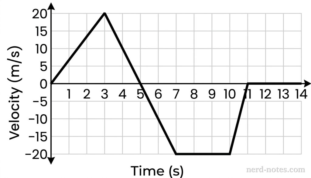
You throw a ball straight upward. It leaves your hand at \( 20 \) \( \text{m/s} \) and slows at a steady rate until it stops at the peak. The ball then comes back down, speeding up steadily until it hits the ground with the same speed it left your hand. Draw the velocity vs. time graph or explain it in terms of functions.
Two identical metal balls are being held side by side at the top of a ramp. Alex lets one ball, \( A \), start rolling down the hill. A few seconds later, Alex’s partner, Bob, starts the second ball, \( B \), down the hill by giving it a push. Ball \( B \) rolls down an identical, parallel path to the first ball and passes it. At the instant ball \( B \) passes ball \( A \) (select all that apply):
A car decelerates from \( 25 \, \text{m/s} \) to \( 5 \, \text{m/s} \) at \( 10 \, \text{m/s}^2 \). How far does the car travel during this deceleration?
In which of the following is the rate of change of the particle’s momentum zero?
Which pair of quantities will always have the same magnitude if motion is in a straight line and in one direction?
A projectile is launched at \( 25 \) \( \text{m/s} \) at an angle of \( 37^{\circ} \). It lands on a platform that is \( 5.0 \) \( \text{m} \) above the launch height.
Why is the stopping distance of a truck much shorter than for a train going the same speed? Hint: try deriving a formula or stopping distance.
A ball is thrown straight up. What are the velocity and acceleration of the ball at the highest point in its path?
A) \( 2.92 \, \text{s} \)
B) \( -26.62 \, \text{m/s} \)
By continuing you (1) agree to our Terms of Use and Terms of Sale and (2) consent to sharing your IP and browser information used by this site’s security protocols as outlined in our Privacy Policy.
| Kinematics | Forces |
|---|---|
| \(\Delta x = v_i t + \frac{1}{2} at^2\) | \(F = ma\) |
| \(v = v_i + at\) | \(F_g = \frac{G m_1 m_2}{r^2}\) |
| \(v^2 = v_i^2 + 2a \Delta x\) | \(f = \mu N\) |
| \(\Delta x = \frac{v_i + v}{2} t\) | \(F_s =-kx\) |
| \(v^2 = v_f^2 \,-\, 2a \Delta x\) |
| Circular Motion | Energy |
|---|---|
| \(F_c = \frac{mv^2}{r}\) | \(KE = \frac{1}{2} mv^2\) |
| \(a_c = \frac{v^2}{r}\) | \(PE = mgh\) |
| \(T = 2\pi \sqrt{\frac{r}{g}}\) | \(KE_i + PE_i = KE_f + PE_f\) |
| \(W = Fd \cos\theta\) |
| Momentum | Torque and Rotations |
|---|---|
| \(p = mv\) | \(\tau = r \cdot F \cdot \sin(\theta)\) |
| \(J = \Delta p\) | \(I = \sum mr^2\) |
| \(p_i = p_f\) | \(L = I \cdot \omega\) |
| Simple Harmonic Motion | Fluids |
|---|---|
| \(F = -kx\) | \(P = \frac{F}{A}\) |
| \(T = 2\pi \sqrt{\frac{l}{g}}\) | \(P_{\text{total}} = P_{\text{atm}} + \rho gh\) |
| \(T = 2\pi \sqrt{\frac{m}{k}}\) | \(Q = Av\) |
| \(x(t) = A \cos(\omega t + \phi)\) | \(F_b = \rho V g\) |
| \(a = -\omega^2 x\) | \(A_1v_1 = A_2v_2\) |
| Constant | Description |
|---|---|
| [katex]g[/katex] | Acceleration due to gravity, typically [katex]9.8 , \text{m/s}^2[/katex] on Earth’s surface |
| [katex]G[/katex] | Universal Gravitational Constant, [katex]6.674 \times 10^{-11} , \text{N} \cdot \text{m}^2/\text{kg}^2[/katex] |
| [katex]\mu_k[/katex] and [katex]\mu_s[/katex] | Coefficients of kinetic ([katex]\mu_k[/katex]) and static ([katex]\mu_s[/katex]) friction, dimensionless. Static friction ([katex]\mu_s[/katex]) is usually greater than kinetic friction ([katex]\mu_k[/katex]) as it resists the start of motion. |
| [katex]k[/katex] | Spring constant, in [katex]\text{N/m}[/katex] |
| [katex] M_E = 5.972 \times 10^{24} , \text{kg} [/katex] | Mass of the Earth |
| [katex] M_M = 7.348 \times 10^{22} , \text{kg} [/katex] | Mass of the Moon |
| [katex] M_M = 1.989 \times 10^{30} , \text{kg} [/katex] | Mass of the Sun |
| Variable | SI Unit |
|---|---|
| [katex]s[/katex] (Displacement) | [katex]\text{meters (m)}[/katex] |
| [katex]v[/katex] (Velocity) | [katex]\text{meters per second (m/s)}[/katex] |
| [katex]a[/katex] (Acceleration) | [katex]\text{meters per second squared (m/s}^2\text{)}[/katex] |
| [katex]t[/katex] (Time) | [katex]\text{seconds (s)}[/katex] |
| [katex]m[/katex] (Mass) | [katex]\text{kilograms (kg)}[/katex] |
| Variable | Derived SI Unit |
|---|---|
| [katex]F[/katex] (Force) | [katex]\text{newtons (N)}[/katex] |
| [katex]E[/katex], [katex]PE[/katex], [katex]KE[/katex] (Energy, Potential Energy, Kinetic Energy) | [katex]\text{joules (J)}[/katex] |
| [katex]P[/katex] (Power) | [katex]\text{watts (W)}[/katex] |
| [katex]p[/katex] (Momentum) | [katex]\text{kilogram meters per second (kgm/s)}[/katex] |
| [katex]\omega[/katex] (Angular Velocity) | [katex]\text{radians per second (rad/s)}[/katex] |
| [katex]\tau[/katex] (Torque) | [katex]\text{newton meters (Nm)}[/katex] |
| [katex]I[/katex] (Moment of Inertia) | [katex]\text{kilogram meter squared (kgm}^2\text{)}[/katex] |
| [katex]f[/katex] (Frequency) | [katex]\text{hertz (Hz)}[/katex] |
Metric Prefixes
Example of using unit analysis: Convert 5 kilometers to millimeters.
Start with the given measurement: [katex]\text{5 km}[/katex]
Use the conversion factors for kilometers to meters and meters to millimeters: [katex]\text{5 km} \times \frac{10^3 \, \text{m}}{1 \, \text{km}} \times \frac{10^3 \, \text{mm}}{1 \, \text{m}}[/katex]
Perform the multiplication: [katex]\text{5 km} \times \frac{10^3 \, \text{m}}{1 \, \text{km}} \times \frac{10^3 \, \text{mm}}{1 \, \text{m}} = 5 \times 10^3 \times 10^3 \, \text{mm}[/katex]
Simplify to get the final answer: [katex]\boxed{5 \times 10^6 \, \text{mm}}[/katex]
Prefix | Symbol | Power of Ten | Equivalent |
|---|---|---|---|
Pico- | p | [katex]10^{-12}[/katex] | 0.000000000001 |
Nano- | n | [katex]10^{-9}[/katex] | 0.000000001 |
Micro- | µ | [katex]10^{-6}[/katex] | 0.000001 |
Milli- | m | [katex]10^{-3}[/katex] | 0.001 |
Centi- | c | [katex]10^{-2}[/katex] | 0.01 |
Deci- | d | [katex]10^{-1}[/katex] | 0.1 |
(Base unit) | – | [katex]10^{0}[/katex] | 1 |
Deca- or Deka- | da | [katex]10^{1}[/katex] | 10 |
Hecto- | h | [katex]10^{2}[/katex] | 100 |
Kilo- | k | [katex]10^{3}[/katex] | 1,000 |
Mega- | M | [katex]10^{6}[/katex] | 1,000,000 |
Giga- | G | [katex]10^{9}[/katex] | 1,000,000,000 |
Tera- | T | [katex]10^{12}[/katex] | 1,000,000,000,000 |
One price to unlock most advanced version of Phy across all our tools.
per month
Billed Monthly. Cancel Anytime.
Try our free calculator to see what you need to get a 5 on the 2026 AP Physics 1 exam.
A quick explanation
Credits are used to grade your FRQs and GQs. Pro users get unlimited credits.
Submitting counts as 1 attempt.
Viewing answers or explanations count as a failed attempts.
Phy gives partial credit if needed
MCQs and GQs are are 1 point each. FRQs will state points for each part.
Phy customizes problem explanations based on what you struggle with. Just hit the explanation button to see.
Understand you mistakes quicker.

Phy automatically provides feedback so you can improve your responses.
10 Free Credits To Get You Started

By continuing you agree to nerd-notes.com Terms of Service, Privacy Policy, and our usage of user data.
Feeling uneasy about your next physics test? We'll boost your grade in 3 lessons or less—guaranteed

NEW! PHY AI accurately solves all questions
🔥 Get up to 30% off Elite Physics Tutoring
🧠 NEW! Learn Physics From Scratch Self Paced Course
🎯 Need exam style practice questions?