
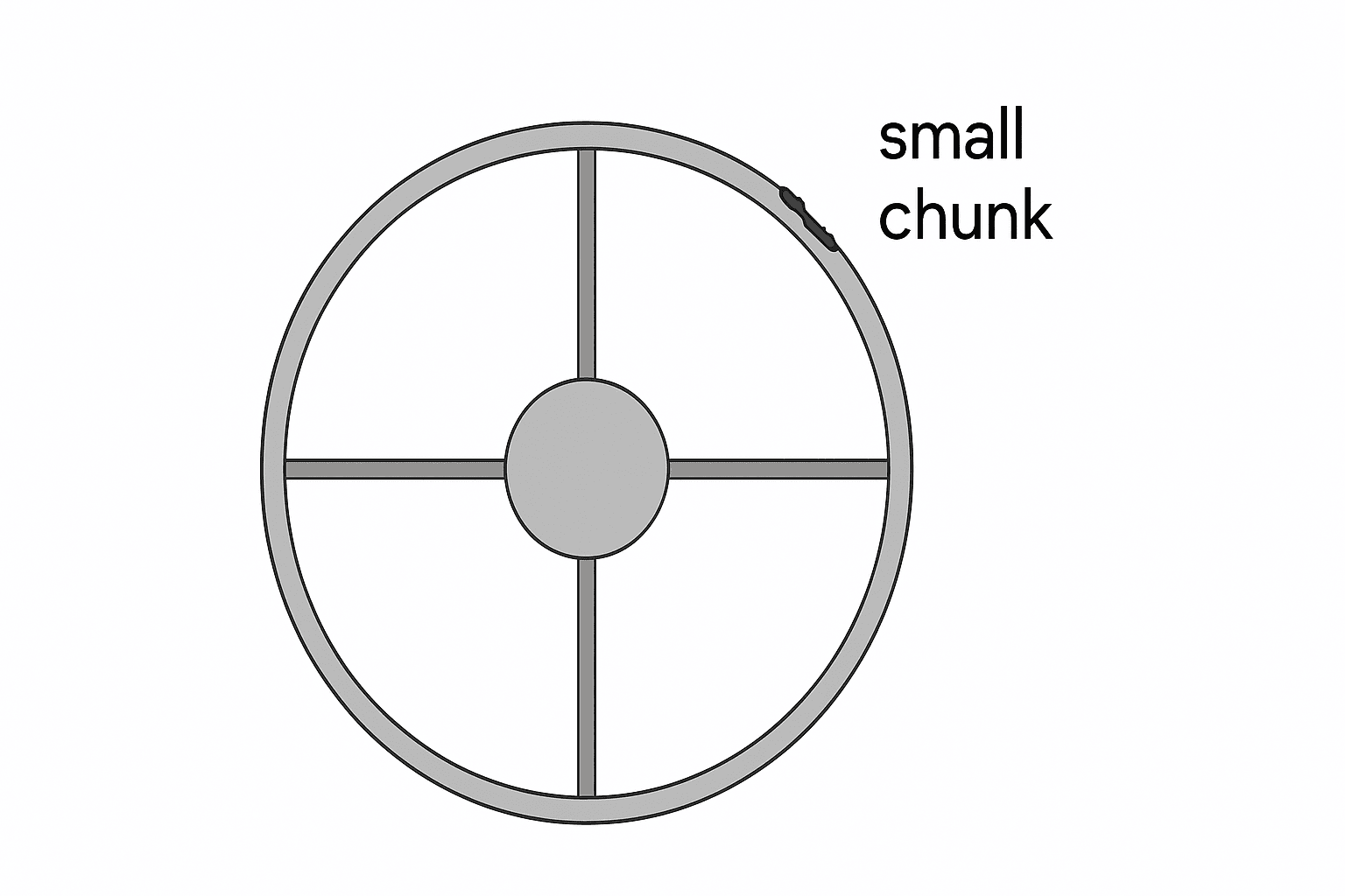
The object shown in the diagram below consists of a cylinder of mass \( 100 \) \( \text{kg} \) and radius \( 25.0 \) \( \text{cm} \) connected by four thin rods, each of mass \( 5.00 \) \( \text{kg} \) and length \( 0.75 \) \( \text{m} \), to a thin-outer ring of mass \( 20.0 \) \( \text{kg} \). A small chunk of metal of mass \( 1.00 \) \( \text{kg} \) is welded to the outer ring. Determine the moment of inertia of the entire assembly about the center of the inner cylinder, treating the metal chunk as a point mass. Hint: The moment of inertia of a disk about it center is \(\tfrac{1}{2} M R^2\), a thin rod about it center is \(\tfrac{1}{12}ML^2\), and a thin hoop about its center is \(I = MR^2\).

A point on the edge of a disk rotates around the center of the disk with an initial angular velocity of 3 rad/s clockwise. The graph shows the point’s angular acceleration as a function of time. The positive direction is considered to be counterclockwise. All frictional forces are considered to be negligible.
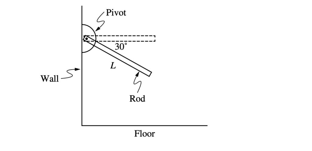
A uniform rod of mass \( M_0 \) and length \( L \) is free to rotate about a pivot at its left end and is released from rest when the rod is \( 30^{\circ} \) below the horizontal, as shown in the figure. With respect to the pivot, the rod has rotational inertia \( I_0 = \dfrac{1}{3} M_0 L^2 \). Which of the following expressions correctly represents the magnitude of the net torque exerted on the rod about the pivot at the moment the rod is released?


