
A rod is initially at rest on a rough horizontal surface. Three forces are exerted on the rod with the magnitudes and directions shown in the figure. The force exerted in the center of the rod is an equidistant 0.5 m from both ends of the rod. If friction between the rod and the table prevents the rod from rotating, what is the magnitude of the torque exerted on the rod about its center from frictional forces?

In lacrosse, a typical throw is made by rotating the stick through an angle of roughly \(90^\circ\), then releasing the ball when the stick is vertical, as shown above. If the \(1 \, \text{meter}\) long stick is at rest when horizontal and the ball leaves the stick with a velocity of \(10 \, \text{m/s}\), what angular acceleration must the stick experience?
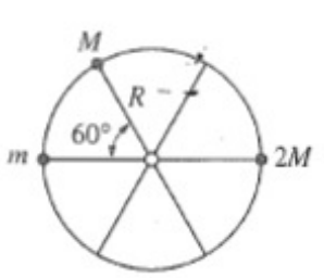
A wheel of radius \( R \) and negligible mass is mounted on a horizontal frictionless axle so that the wheel is in a vertical plane. Three small objects having masses \( m \), \( M \), and \( 2M \), respectively, are mounted on the rim of the wheel, as shown above. If the system is in static equilibrium, what is the value of \( m \) in terms of \( M \)?


