| Step | Reasoning |
|---|---|
| Identify the target equation for torque magnitude. \[ \tau = rF\sin\theta \] |
The question asks to rank torque magnitudes based on varied distance, force, and angle. |
| Calculate the torque for Scenario I. \[ \tau_I = L \cdot F \cdot \sin(90^\circ) = LF(1) = LF \] |
This serves as the baseline for comparison using the provided variables. |
| Calculate the torque for Scenario II. \[ \tau_{II} = 2L \cdot F \cdot \sin(30^\circ) = 2LF(0.5) = LF \] |
To compare a force applied at a larger distance with an angle. |
| Calculate the torque for Scenario III. \[ \tau_{III} = L \cdot \left(\dfrac{F}{2}\right) \cdot \sin(90^\circ) = 0.5LF \] |
To compare the effect of reduced force magnitude. |
| Calculate the torque for Scenario IV. \[ \tau_{IV} = \left(\dfrac{L}{2}\right) \cdot 2F \cdot \sin(30^\circ) = LF(0.5) = 0.5LF \] |
To compare the combined effect of increased force, decreased distance, and an angle. |
| Compare the calculated values to determine the final ranking. \[ LF = LF > 0.5LF = 0.5LF \] |
Combining the results of the previous steps leads to the correct choice. |
Why each choice is correct or incorrect:
(A) This is the correct answer based on evaluating the torque equation for each scenario.
(B) This ranking results from miscalculating the value of sin(30) as being larger than 0.5 or ignoring it for Scenario II.
(C) This suggests a misunderstanding of how the sine function scales the torque; the values in III and IV are exactly half those in I and II.
(D) This occurs if the sin(theta) term is ignored entirely, treating every scenario as if the force were applied perpendicularly.
A Major Upgrade To Phy Is Coming Soon — Stay Tuned
We'll help clarify entire units in one hour or less — guaranteed.
A self paced course with videos, problems sets, and everything you need to get a 5. Trusted by over 15k students and over 200 schools.

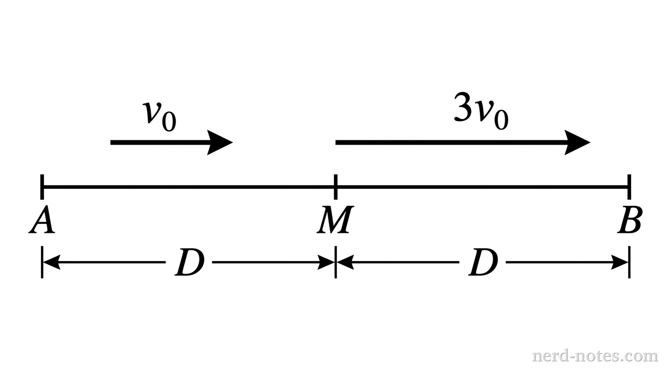
A car travels along a straight road between two cities separated by a total distance of \(2D\). The car travels the first distance \(D\) at a constant speed \(v_0\) and the remaining distance \(D\) at a constant speed \(3v_0\). Which of the following correctly identifies the average speed \(v_{avg}\) of the car for the entire trip and provides a valid justification?

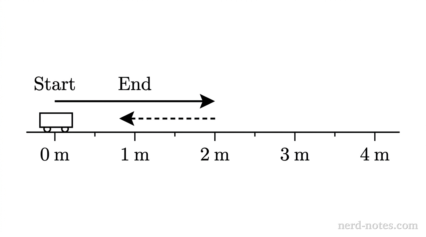
A student conducts a laboratory experiment where a cart is moved \(2.0 \text{ m}\) to the right and then \(1.0 \text{ m}\) to the left along a straight, horizontal track. The student calculates the total distance traveled and the final displacement of the cart. Which of the following correctly classifies these quantities and provides a valid justification?

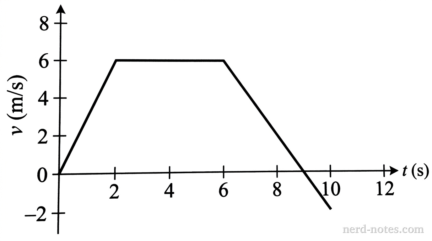
An experimental automated cart is tested on a linear track. A computer-controlled sensor measures the cart’s velocity \(v\) as a function of time \(t\), as shown in the graph. What is the displacement of the cart during the time interval from \(t = 0 \text{ s}\) to \(t = 10 \text{ s}\)?

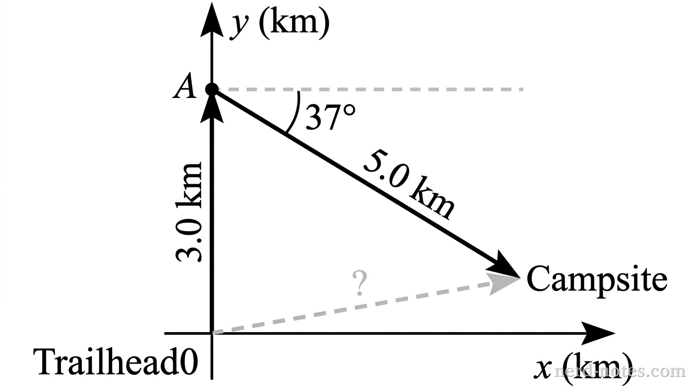
A hiker starts at a trailhead and walks \(3.0 \text{ km}\) due North. The hiker then turns and walks \(5.0 \text{ km}\) in a direction \(37^\circ\) South of East to reach a campsite. (Note: \(\sin 37^\circ \approx 0.60\); \(\cos 37^\circ \approx 0.80\)). What is the magnitude of the hiker’s total displacement from the trailhead to the campsite?

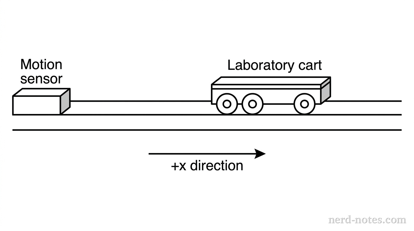
A laboratory cart is restricted to motion along a horizontal track. A motion sensor records the direction of the cart’s velocity and the direction of its acceleration at three different times, as shown in the table below.
| Time | Direction of Velocity | Direction of Acceleration |
| :— | :— | :— |
| \(t_1\) | Right | Left |
| \(t_2\) | Left | Left |
| \(t_3\) | Left | Right |
Which of the following correctly describes the motion of the cart at each time?

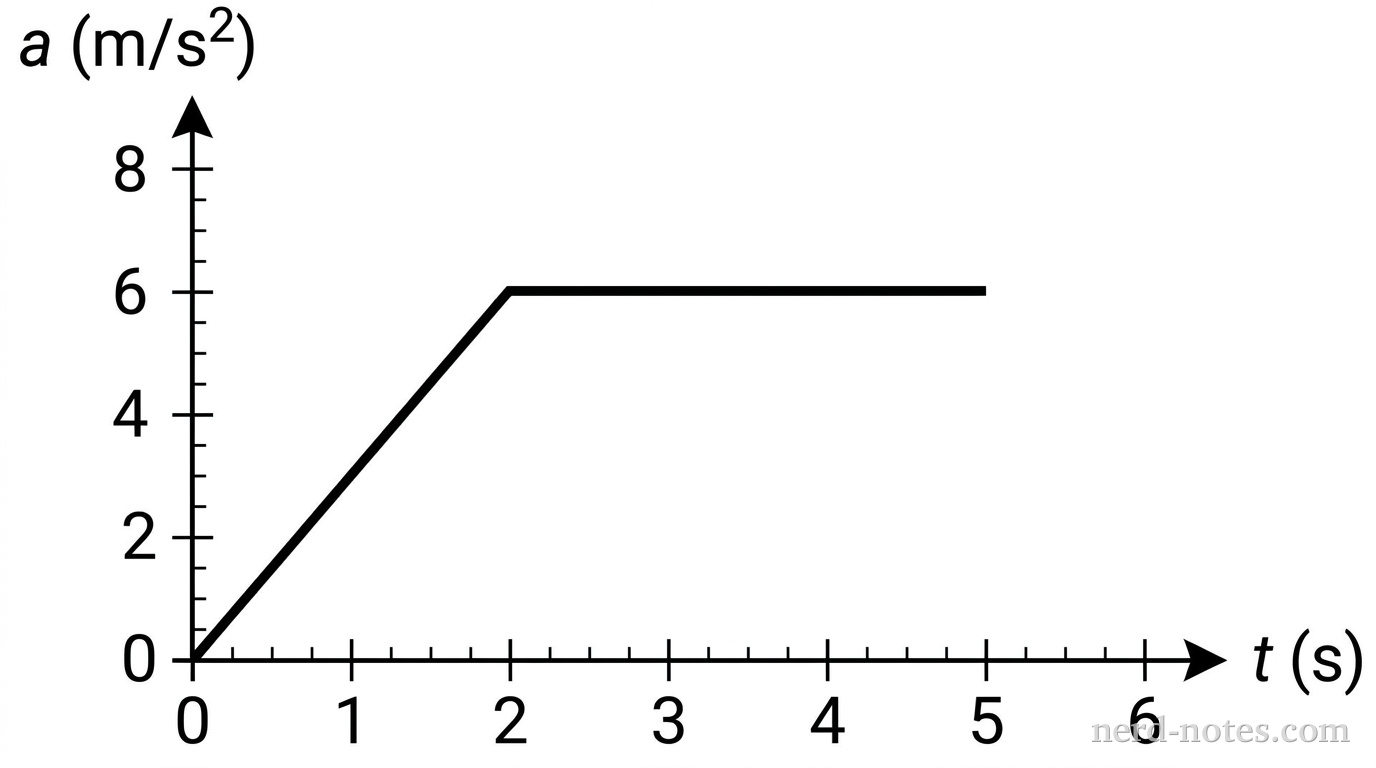
A test rocket moves along a straight, horizontal track. A sensor records the rocket’s acceleration as a function of time, as shown in the graph below.
What is the average acceleration of the rocket during the time interval from \(t = 0 \text{ s}\) to \(t = 5 \text{ s}\)?

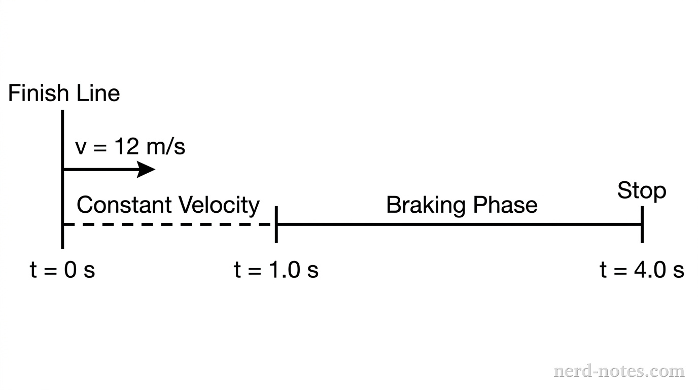
A sprinter crosses the finish line of a race moving with a velocity of \(12 \text{ m/s}\). The sprinter continues to run at this constant velocity for a reaction time of \(1.0 \text{ s}\) before beginning to slow down with a constant acceleration. If the sprinter comes to a complete stop exactly \(4.0 \text{ s}\) after crossing the finish line, what is the magnitude of the sprinter’s acceleration during the braking phase?

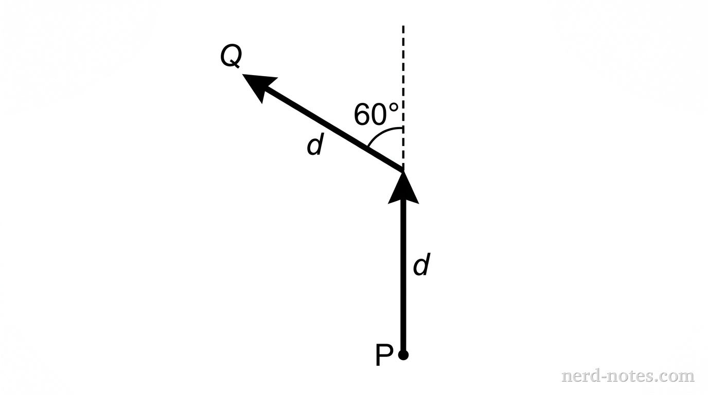
A surveyor starts at point \(P\) and walks a distance \(d\) due north. The surveyor then turns and walks an equal distance \(d\) in a direction \(60^{\circ}\) west of north to reach point \(Q\). What is the magnitude of the surveyor’s total displacement from point \(P\) to point \(Q\)?

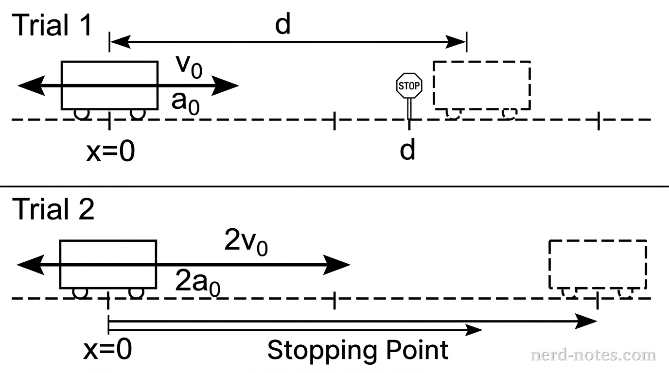
A train is traveling at a constant speed \( v_0 \) when the engineer applies the brakes, resulting in a constant deceleration of magnitude \( a_0 \) that brings the train to a stop in a distance \( d \). In a second trial, the train is traveling at a speed \( 2v_0 \) when the brakes are applied and is brought to a stop with a constant deceleration of magnitude \( 2a_0 \). Which of the following is the stopping distance for the train in the second trial?

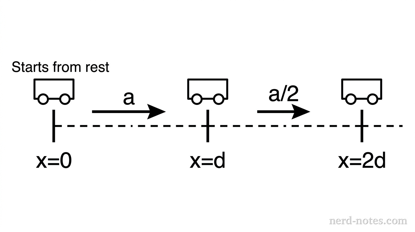
A small experimental vehicle starts from rest and accelerates with a constant acceleration \(a\) over a horizontal distance \(d\). After this distance, the vehicle’s engine is adjusted such that it continues to accelerate at a constant rate of \(\dfrac{a}{2}\) for an additional horizontal distance \(d\). Which of the following expressions represents the speed of the vehicle after it has traveled the total distance \(2d\)?
A
By continuing you (1) agree to our Terms of Use and Terms of Sale and (2) consent to sharing your IP and browser information used by this site’s security protocols as outlined in our Privacy Policy.
| Kinematics | Forces |
|---|---|
| \(\Delta x = v_i t + \frac{1}{2} at^2\) | \(F = ma\) |
| \(v = v_i + at\) | \(F_g = \frac{G m_1 m_2}{r^2}\) |
| \(v^2 = v_i^2 + 2a \Delta x\) | \(f = \mu N\) |
| \(\Delta x = \frac{v_i + v}{2} t\) | \(F_s =-kx\) |
| \(v^2 = v_f^2 \,-\, 2a \Delta x\) |
| Circular Motion | Energy |
|---|---|
| \(F_c = \frac{mv^2}{r}\) | \(KE = \frac{1}{2} mv^2\) |
| \(a_c = \frac{v^2}{r}\) | \(PE = mgh\) |
| \(T = 2\pi \sqrt{\frac{r}{g}}\) | \(KE_i + PE_i = KE_f + PE_f\) |
| \(W = Fd \cos\theta\) |
| Momentum | Torque and Rotations |
|---|---|
| \(p = mv\) | \(\tau = r \cdot F \cdot \sin(\theta)\) |
| \(J = \Delta p\) | \(I = \sum mr^2\) |
| \(p_i = p_f\) | \(L = I \cdot \omega\) |
| Simple Harmonic Motion | Fluids |
|---|---|
| \(F = -kx\) | \(P = \frac{F}{A}\) |
| \(T = 2\pi \sqrt{\frac{l}{g}}\) | \(P_{\text{total}} = P_{\text{atm}} + \rho gh\) |
| \(T = 2\pi \sqrt{\frac{m}{k}}\) | \(Q = Av\) |
| \(x(t) = A \cos(\omega t + \phi)\) | \(F_b = \rho V g\) |
| \(a = -\omega^2 x\) | \(A_1v_1 = A_2v_2\) |
| Constant | Description |
|---|---|
| [katex]g[/katex] | Acceleration due to gravity, typically [katex]9.8 , \text{m/s}^2[/katex] on Earth’s surface |
| [katex]G[/katex] | Universal Gravitational Constant, [katex]6.674 \times 10^{-11} , \text{N} \cdot \text{m}^2/\text{kg}^2[/katex] |
| [katex]\mu_k[/katex] and [katex]\mu_s[/katex] | Coefficients of kinetic ([katex]\mu_k[/katex]) and static ([katex]\mu_s[/katex]) friction, dimensionless. Static friction ([katex]\mu_s[/katex]) is usually greater than kinetic friction ([katex]\mu_k[/katex]) as it resists the start of motion. |
| [katex]k[/katex] | Spring constant, in [katex]\text{N/m}[/katex] |
| [katex] M_E = 5.972 \times 10^{24} , \text{kg} [/katex] | Mass of the Earth |
| [katex] M_M = 7.348 \times 10^{22} , \text{kg} [/katex] | Mass of the Moon |
| [katex] M_M = 1.989 \times 10^{30} , \text{kg} [/katex] | Mass of the Sun |
| Variable | SI Unit |
|---|---|
| [katex]s[/katex] (Displacement) | [katex]\text{meters (m)}[/katex] |
| [katex]v[/katex] (Velocity) | [katex]\text{meters per second (m/s)}[/katex] |
| [katex]a[/katex] (Acceleration) | [katex]\text{meters per second squared (m/s}^2\text{)}[/katex] |
| [katex]t[/katex] (Time) | [katex]\text{seconds (s)}[/katex] |
| [katex]m[/katex] (Mass) | [katex]\text{kilograms (kg)}[/katex] |
| Variable | Derived SI Unit |
|---|---|
| [katex]F[/katex] (Force) | [katex]\text{newtons (N)}[/katex] |
| [katex]E[/katex], [katex]PE[/katex], [katex]KE[/katex] (Energy, Potential Energy, Kinetic Energy) | [katex]\text{joules (J)}[/katex] |
| [katex]P[/katex] (Power) | [katex]\text{watts (W)}[/katex] |
| [katex]p[/katex] (Momentum) | [katex]\text{kilogram meters per second (kgm/s)}[/katex] |
| [katex]\omega[/katex] (Angular Velocity) | [katex]\text{radians per second (rad/s)}[/katex] |
| [katex]\tau[/katex] (Torque) | [katex]\text{newton meters (Nm)}[/katex] |
| [katex]I[/katex] (Moment of Inertia) | [katex]\text{kilogram meter squared (kgm}^2\text{)}[/katex] |
| [katex]f[/katex] (Frequency) | [katex]\text{hertz (Hz)}[/katex] |
Metric Prefixes
Example of using unit analysis: Convert 5 kilometers to millimeters.
Start with the given measurement: [katex]\text{5 km}[/katex]
Use the conversion factors for kilometers to meters and meters to millimeters: [katex]\text{5 km} \times \frac{10^3 \, \text{m}}{1 \, \text{km}} \times \frac{10^3 \, \text{mm}}{1 \, \text{m}}[/katex]
Perform the multiplication: [katex]\text{5 km} \times \frac{10^3 \, \text{m}}{1 \, \text{km}} \times \frac{10^3 \, \text{mm}}{1 \, \text{m}} = 5 \times 10^3 \times 10^3 \, \text{mm}[/katex]
Simplify to get the final answer: [katex]\boxed{5 \times 10^6 \, \text{mm}}[/katex]
Prefix | Symbol | Power of Ten | Equivalent |
|---|---|---|---|
Pico- | p | [katex]10^{-12}[/katex] | 0.000000000001 |
Nano- | n | [katex]10^{-9}[/katex] | 0.000000001 |
Micro- | µ | [katex]10^{-6}[/katex] | 0.000001 |
Milli- | m | [katex]10^{-3}[/katex] | 0.001 |
Centi- | c | [katex]10^{-2}[/katex] | 0.01 |
Deci- | d | [katex]10^{-1}[/katex] | 0.1 |
(Base unit) | – | [katex]10^{0}[/katex] | 1 |
Deca- or Deka- | da | [katex]10^{1}[/katex] | 10 |
Hecto- | h | [katex]10^{2}[/katex] | 100 |
Kilo- | k | [katex]10^{3}[/katex] | 1,000 |
Mega- | M | [katex]10^{6}[/katex] | 1,000,000 |
Giga- | G | [katex]10^{9}[/katex] | 1,000,000,000 |
Tera- | T | [katex]10^{12}[/katex] | 1,000,000,000,000 |
One price to unlock most advanced version of Phy across all our tools.
per month
Billed Monthly. Cancel Anytime.
We crafted THE Ultimate A.P Physics 1 Program so you can learn faster and score higher.
Try our free calculator to see what you need to get a 5 on the 2026 AP Physics 1 exam.
A quick explanation
Credits are used to grade your FRQs and GQs. Pro users get unlimited credits.
Submitting counts as 1 attempt.
Viewing answers or explanations count as a failed attempts.
Phy gives partial credit if needed
MCQs and GQs are are 1 point each. FRQs will state points for each part.
Phy customizes problem explanations based on what you struggle with. Just hit the explanation button to see.
Understand you mistakes quicker.
Phy automatically provides feedback so you can improve your responses.
10 Free Credits To Get You Started
By continuing you agree to nerd-notes.com Terms of Service, Privacy Policy, and our usage of user data.
Feeling uneasy about your next physics test? We'll boost your grade in 3 lessons or less—guaranteed
NEW! PHY AI accurately solves all questions
🔥 Get up to 30% off Elite Physics Tutoring
🧠 NEW! Learn Physics From Scratch Self Paced Course
🎯 Need exam style practice questions?