Part (a) – Finding the orbital speed.
| Step | Derivation/Formula | Reasoning |
|---|---|---|
| 1 | [katex] r = \frac{50}{2} = 25 \text{km} = 25000 \text{m} [/katex] | The radius [katex] r [/katex] of the orbit is half the diameter. Convert it to meters. |
| 2 | [katex] T = 11 \times 86400 [/katex] s | Convert period [katex] T [/katex] from days to seconds. There are 86400 seconds in a day. |
| 3 | [katex] v = \frac{2\pi r}{T} [/katex] | The orbital speed [katex] v [/katex] is calculated by dividing the circumference of the orbit by the orbital period. |
| 4 | [katex] v = \frac{2\pi \times 25000}{950400} [/katex] m/s | Substitute the values of [katex] r [/katex] and [katex] T [/katex] into the formula. Convert [katex] r [/katex] from km to m by multiplying by 1000. |
| 5 | [katex] v \approx 0.165 [/katex] m/s | Simplifying the expression gives the orbital speed [katex] v [/katex]. |
| 6 | [katex] \boxed{v \approx 0.165 \text{m/s}} [/katex] | This is the final value for the satellite’s orbital speed. |
Part (b) – Finding the comet’s mass.
| Step | Derivation/Formula | Reasoning |
|---|---|---|
| 1 | [katex] v^2 = \frac{GM}{r} [/katex] | The inwards gravitational force is equal to the centripetal force of the orbiting comet. In terms of Newtons law this can be expressed as [katex]\frac{GMm}{r^2} = \frac{mv^2}{r} [/katex], where [katex] M [/katex] is the mass of the comet, [katex] m [/katex] [katex] is the mass of the satellite, and G [/katex] is the gravitational constant. |
| 2 | [katex] M = \frac{rv^2}{G} [/katex] | Rearrange the formula to solve for the mass [katex] M [/katex] of the comet. |
| 3 | [katex] M = \frac{25000 \times (0.165)^2}{6.674 \times 10^{-11}} [/katex] kg | Substitute the values of [katex] r [/katex] and [katex] v [/katex] into the formula, remembering that [katex] r [/katex] is already converted to meters. |
| 4 | [katex] M \approx 1.02 \times 10^{13} [/katex] kg | Calculating the value gives the mass of the comet. |
| 5 | [katex] \boxed{M \approx 1.02 \times 10^{13} \text{kg}} [/katex] | This is the final value for the mass of the comet. |
Part (c) – Finding the landing speed.
| Step | Derivation/Formula | Reasoning |
|---|---|---|
| 1 | [katex] h = 25\,\text{km}\, -\,1.8 \, \text{km} = 23.2 \, \text{km} = 23200 \, \text{meters} [/katex] | The distance from the satellite to the center of the comet is 25km. Since the comet has an average diameter of 3.6 km (or a radius of 1.8 km). The distance from the satellite to the surface of comet is 23.2 km. Convert this to meters. |
| 2 | [katex] t = 7 \times 3600 [/katex] s | Convert the fall time [katex] t [/katex] from hours to seconds. |
| 3 | [katex] g = \frac{GM}{r^2} [/katex] | Calculate the acceleration [katex] g [/katex] due to the comet’s gravity using the values from the previous two parts. Set [katex] mg = \frac{GMm}{r^2} [/katex] and solve for [katex] g [/katex]. |
| 4 | [katex] g = \frac{(6.67\times 10^{-11}) \times (1.02 \times 10^{13})}{25000^2} [/katex] | Substitute values into the equation for gravitational acceleration. |
| 5 | [katex] g = 1.09 \times 10^{-6} \, \text{m/s}^2 [/katex] | Final value for [katex]g [/katex],the acceleration due to gravity of the comet. |
| 6 | [katex] v^2_{\text{final}} = v^2_{\text{initial}} + 2a\Delta x [/katex] | Now that we have [katex] v_{initial}, \, a, \, \Delta x [/katex] we can use a kinematic formula to solve for [katex] v_f [/katex]. |
| 7 | [katex] \boxed{v_{\text{final}} \approx .735\, \text{m/s}} [/katex] | Plug in all known values and solve for [katex] v_f [/katex]. |
A Major Upgrade To Phy Is Coming Soon — Stay Tuned
We'll help clarify entire units in one hour or less — guaranteed.
A box rests on the (frictionless) bed of a truck. The truck driver starts the truck and accelerates forward. The box immediately starts to slide toward the rear of the truck bed.
A 2.00 x10² g block on a 50.0 cm long string swings in a circle on a horizontal, frictionless table at 75.0 rpm. What is the speed of block? What is the tension in the string?
A car can decelerate at \( -3.80 \, \text{m/s}^2 \) without skidding when coming to rest on a level road. What would its deceleration be if the road is inclined at \( 9.3^\circ \) and the car moves uphill? Assume the same static friction coefficient.
A runner pushes against the track to sprint forward. Which two action–reaction FORCE pairs are involved? Select two letters.
A westward–moving car is changing its speed. The net force on the car ____.
A horizontal \( 300 \) \( \text{N} \) force pushes a \( 40 \) \( \text{kg} \) object across a horizontal \( 10 \) \( \text{meter} \) frictionless surface. After this, the block slides up a \( 20^\circ \) incline. Assuming the incline has a coefficient of kinetic friction of \( 0.4 \), how far along the incline will the object slide?
A person stands on a scale in an elevator. If the scale reads \( 600 \, \text{N} \) when that person is riding upward at a constant velocity of \( 4 \, \text{m/s} \), what is the scale reading when the elevator is at rest? Hint: The reading on the scale is simply the normal force.
A car is safely negotiating an unbanked circular turn at a speed of \(17 \, \text{m/s}\) on dry road. However, a long wet patch in the road appears and decreases the maximum static frictional force to one-fifth of its dry-road value. If the car is to continue safely around the curve, by what factor would the it need to change the original velocity?
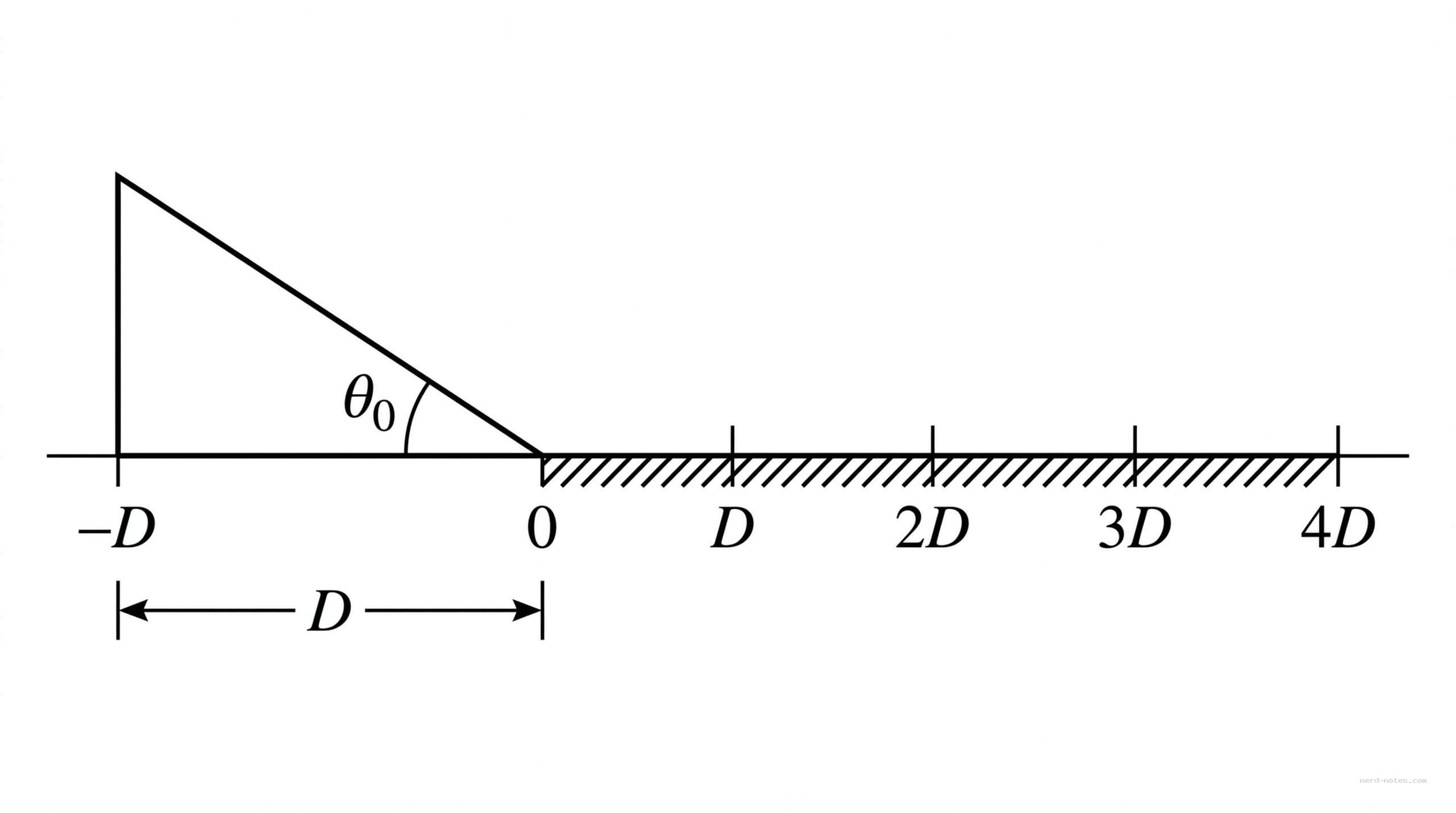
A block is initially at rest on top of an inclined ramp that makes an angle \( \theta_0 \) with the horizontal. The distance measured along the base of the ramp is \( D \). After the block is released from rest, it slides down the frictionless ramp and then continues onto a rough horizontal surface until it finally comes to rest at the position \( x = 4D \) measured from the base of the ramp. The coefficient of kinetic friction between the block and the rough horizontal surface is \( \mu_k \).
An object has a mass of 10 kg. For each case below answer the questions and provide an example.
By continuing you (1) agree to our Terms of Use and Terms of Sale and (2) consent to sharing your IP and browser information used by this site’s security protocols as outlined in our Privacy Policy.
| Kinematics | Forces |
|---|---|
| \(\Delta x = v_i t + \frac{1}{2} at^2\) | \(F = ma\) |
| \(v = v_i + at\) | \(F_g = \frac{G m_1 m_2}{r^2}\) |
| \(v^2 = v_i^2 + 2a \Delta x\) | \(f = \mu N\) |
| \(\Delta x = \frac{v_i + v}{2} t\) | \(F_s =-kx\) |
| \(v^2 = v_f^2 \,-\, 2a \Delta x\) |
| Circular Motion | Energy |
|---|---|
| \(F_c = \frac{mv^2}{r}\) | \(KE = \frac{1}{2} mv^2\) |
| \(a_c = \frac{v^2}{r}\) | \(PE = mgh\) |
| \(T = 2\pi \sqrt{\frac{r}{g}}\) | \(KE_i + PE_i = KE_f + PE_f\) |
| \(W = Fd \cos\theta\) |
| Momentum | Torque and Rotations |
|---|---|
| \(p = mv\) | \(\tau = r \cdot F \cdot \sin(\theta)\) |
| \(J = \Delta p\) | \(I = \sum mr^2\) |
| \(p_i = p_f\) | \(L = I \cdot \omega\) |
| Simple Harmonic Motion | Fluids |
|---|---|
| \(F = -kx\) | \(P = \frac{F}{A}\) |
| \(T = 2\pi \sqrt{\frac{l}{g}}\) | \(P_{\text{total}} = P_{\text{atm}} + \rho gh\) |
| \(T = 2\pi \sqrt{\frac{m}{k}}\) | \(Q = Av\) |
| \(x(t) = A \cos(\omega t + \phi)\) | \(F_b = \rho V g\) |
| \(a = -\omega^2 x\) | \(A_1v_1 = A_2v_2\) |
| Constant | Description |
|---|---|
| [katex]g[/katex] | Acceleration due to gravity, typically [katex]9.8 , \text{m/s}^2[/katex] on Earth’s surface |
| [katex]G[/katex] | Universal Gravitational Constant, [katex]6.674 \times 10^{-11} , \text{N} \cdot \text{m}^2/\text{kg}^2[/katex] |
| [katex]\mu_k[/katex] and [katex]\mu_s[/katex] | Coefficients of kinetic ([katex]\mu_k[/katex]) and static ([katex]\mu_s[/katex]) friction, dimensionless. Static friction ([katex]\mu_s[/katex]) is usually greater than kinetic friction ([katex]\mu_k[/katex]) as it resists the start of motion. |
| [katex]k[/katex] | Spring constant, in [katex]\text{N/m}[/katex] |
| [katex] M_E = 5.972 \times 10^{24} , \text{kg} [/katex] | Mass of the Earth |
| [katex] M_M = 7.348 \times 10^{22} , \text{kg} [/katex] | Mass of the Moon |
| [katex] M_M = 1.989 \times 10^{30} , \text{kg} [/katex] | Mass of the Sun |
| Variable | SI Unit |
|---|---|
| [katex]s[/katex] (Displacement) | [katex]\text{meters (m)}[/katex] |
| [katex]v[/katex] (Velocity) | [katex]\text{meters per second (m/s)}[/katex] |
| [katex]a[/katex] (Acceleration) | [katex]\text{meters per second squared (m/s}^2\text{)}[/katex] |
| [katex]t[/katex] (Time) | [katex]\text{seconds (s)}[/katex] |
| [katex]m[/katex] (Mass) | [katex]\text{kilograms (kg)}[/katex] |
| Variable | Derived SI Unit |
|---|---|
| [katex]F[/katex] (Force) | [katex]\text{newtons (N)}[/katex] |
| [katex]E[/katex], [katex]PE[/katex], [katex]KE[/katex] (Energy, Potential Energy, Kinetic Energy) | [katex]\text{joules (J)}[/katex] |
| [katex]P[/katex] (Power) | [katex]\text{watts (W)}[/katex] |
| [katex]p[/katex] (Momentum) | [katex]\text{kilogram meters per second (kgm/s)}[/katex] |
| [katex]\omega[/katex] (Angular Velocity) | [katex]\text{radians per second (rad/s)}[/katex] |
| [katex]\tau[/katex] (Torque) | [katex]\text{newton meters (Nm)}[/katex] |
| [katex]I[/katex] (Moment of Inertia) | [katex]\text{kilogram meter squared (kgm}^2\text{)}[/katex] |
| [katex]f[/katex] (Frequency) | [katex]\text{hertz (Hz)}[/katex] |
Metric Prefixes
Example of using unit analysis: Convert 5 kilometers to millimeters.
Start with the given measurement: [katex]\text{5 km}[/katex]
Use the conversion factors for kilometers to meters and meters to millimeters: [katex]\text{5 km} \times \frac{10^3 \, \text{m}}{1 \, \text{km}} \times \frac{10^3 \, \text{mm}}{1 \, \text{m}}[/katex]
Perform the multiplication: [katex]\text{5 km} \times \frac{10^3 \, \text{m}}{1 \, \text{km}} \times \frac{10^3 \, \text{mm}}{1 \, \text{m}} = 5 \times 10^3 \times 10^3 \, \text{mm}[/katex]
Simplify to get the final answer: [katex]\boxed{5 \times 10^6 \, \text{mm}}[/katex]
Prefix | Symbol | Power of Ten | Equivalent |
|---|---|---|---|
Pico- | p | [katex]10^{-12}[/katex] | 0.000000000001 |
Nano- | n | [katex]10^{-9}[/katex] | 0.000000001 |
Micro- | µ | [katex]10^{-6}[/katex] | 0.000001 |
Milli- | m | [katex]10^{-3}[/katex] | 0.001 |
Centi- | c | [katex]10^{-2}[/katex] | 0.01 |
Deci- | d | [katex]10^{-1}[/katex] | 0.1 |
(Base unit) | – | [katex]10^{0}[/katex] | 1 |
Deca- or Deka- | da | [katex]10^{1}[/katex] | 10 |
Hecto- | h | [katex]10^{2}[/katex] | 100 |
Kilo- | k | [katex]10^{3}[/katex] | 1,000 |
Mega- | M | [katex]10^{6}[/katex] | 1,000,000 |
Giga- | G | [katex]10^{9}[/katex] | 1,000,000,000 |
Tera- | T | [katex]10^{12}[/katex] | 1,000,000,000,000 |
One price to unlock most advanced version of Phy across all our tools.
per month
Billed Monthly. Cancel Anytime.
We crafted THE Ultimate A.P Physics 1 Program so you can learn faster and score higher.
Try our free calculator to see what you need to get a 5 on the 2026 AP Physics 1 exam.
A quick explanation
Credits are used to grade your FRQs and GQs. Pro users get unlimited credits.
Submitting counts as 1 attempt.
Viewing answers or explanations count as a failed attempts.
Phy gives partial credit if needed
MCQs and GQs are are 1 point each. FRQs will state points for each part.
Phy customizes problem explanations based on what you struggle with. Just hit the explanation button to see.
Understand you mistakes quicker.

Phy automatically provides feedback so you can improve your responses.
10 Free Credits To Get You Started

By continuing you agree to nerd-notes.com Terms of Service, Privacy Policy, and our usage of user data.
Feeling uneasy about your next physics test? We'll boost your grade in 3 lessons or less—guaranteed

NEW! PHY AI accurately solves all questions
🔥 Get up to 30% off Elite Physics Tutoring
🧠 NEW! Learn Physics From Scratch Self Paced Course
🎯 Need exam style practice questions?
