0 attempts
0% avg
| Derivation/Formula | Reasoning |
|---|---|
| \[ \omega(0) = \omega_0 \] | At \( t=0 \) the disk spins counterclockwise, so \( \omega(0)=\omega_0>0 \) with CCW taken as positive. |
| \[ \tau = FR \] | A tangential force \( F \) applied at radius \( R \) produces torque magnitude \( \tau=FR \); the sign follows the CCW-positive convention. |
| \[ \tau_L = (+20)R \] | The left downward force at \( x=-R \) makes a CCW torque, so \( \tau_L=+20R \). |
| \[ \tau_R = (-40)R \] | The right downward force at \( x=+R \) makes a CW torque, so \( \tau_R=-40R \). |
| \[ \tau_{\text{net}} = \tau_L + \tau_R = (20-40)R = -20R \] | Net torque is CW because \( 40>20 \); hence \( \tau_{\text{net}}<0 \). |
| \[ \alpha = \frac{\tau_{\text{net}}}{I} \] | With constant torques, angular acceleration \( \alpha \) is constant. Since \( I>0 \) and \( \tau_{\text{net}}<0 \), we get \( \alpha<0 \). |
| \[ \omega(t) = \omega_0 + \alpha t \] | For constant \( \alpha \), \( \omega(t) \) is a straight line with slope \( \alpha<0 \), starting at \( \omega_0 \). |
| \[ t_{\text{zero}} = \frac{\omega_0}{|\alpha|} \] | \( \omega(t) \) crosses zero at \( t=\omega_0/|\alpha| \) and becomes negative afterward, indicating reversal to CW. |
| \[ \text{Select (c)} \] | The correct graph must start at \( \omega_0 \) and decrease linearly past zero; this matches option \( \text{(c)} \). |
| Derivation/Formula | Reasoning |
|---|---|
| \[ \text{(a)}:\ \omega(0)=-\omega_0,\ \alpha>0 \] | Starts negative and increases; contradicts \( \omega(0)=\omega_0>0 \) and our \( \alpha<0 \). |
| \[ \text{(b)}:\ \alpha=0 \] | Constant \( \omega \) requires \( \tau_{\text{net}}=0 \), but here \( \tau_{\text{net}}=-20R\ne0 \). |
| \[ \text{(c)}:\ \omega(0)=\omega_0,\ \alpha<0 \] | Decreasing straight line crossing zero, exactly what a constant negative \( \alpha \) produces. Correct. |
| \[ \text{(d)}:\ \text{sign}(\alpha): – \to + \] | V-shape implies \( \alpha \) reverses sign after some time, which would require a changing net torque; our \( \tau_{\text{net}} \) is constant. |
Just ask: "Help me solve this problem."
We'll help clarify entire units in one hour or less — guaranteed.
A centrifuge accelerates uniformly from rest to 15,000 rpm in 240 s. Through how many revolutions did it turn in this time?
In which of the following is the rate of change of the particle’s momentum zero?
Wheels \( A \) and \( B \) are connected by a moving belt and are both free to rotate about their centers. The belt does not slip on the wheels. The radius of Wheel \( B \) is twice the radius of Wheel \( A \). Wheel \( A \) has constant angular speed \( \omega_A \) and Wheel \( B \) has constant angular speed \( \omega_B \). Which of the following correctly relates \( \omega_A \) and \( \omega_B \)?
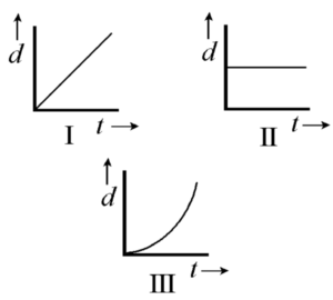
Which graph below shows that one of the runners started 10 meters further ahead of the other? Assume the y-axis is measured in meters and the x-axis is measured in seconds.
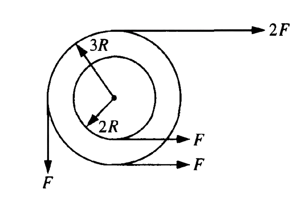
A system of two wheels fixed to each other is free to rotate about a frictionless axis through the common center of the wheels and perpendicular to the page. Four forces are exerted tangentially to the rims of the wheels, as shown in the figure. The magnitude of the net torque on the system about the axis is
A solid disk has a mass \( M \) and radius \( R \). What is the moment of inertia about an axis that is perpendicular to the plane of the disk and passes through its edge? Hint: the moment of inertia about the disk center is given as \(I_{center}=\frac{1}{2}M R^{2}\).
A pulley has an initial angular speed of \( 12.5 \) \( \text{rad/s} \) and a constant angular acceleration of \( 3.41 \) \( \text{rad/s}^2 \). Through what angle does the pulley turn in \( 5.26 \) \( \text{s} \)?
What is the rotational inertia \( I \) of a disk with a radius \( R = 4 \) \( \text{m} \) and a mass \( 2 \) \( \text{kg} \)? The same disk is rotated around an axis that is \( 0.5 \) \( \text{m} \) from the center of the disk. What is the new rotational inertia \( I \) of the disk? What would the rotational inertia be if the disk axis was \( 3.75 \) \( \text{m} \) from the center?
When is the angular momentum of a system constant?
By continuing you (1) agree to our Terms of Use and Terms of Sale and (2) consent to sharing your IP and browser information used by this site’s security protocols as outlined in our Privacy Policy.
| Kinematics | Forces |
|---|---|
| \(\Delta x = v_i t + \frac{1}{2} at^2\) | \(F = ma\) |
| \(v = v_i + at\) | \(F_g = \frac{G m_1 m_2}{r^2}\) |
| \(v^2 = v_i^2 + 2a \Delta x\) | \(f = \mu N\) |
| \(\Delta x = \frac{v_i + v}{2} t\) | \(F_s =-kx\) |
| \(v^2 = v_f^2 \,-\, 2a \Delta x\) |
| Circular Motion | Energy |
|---|---|
| \(F_c = \frac{mv^2}{r}\) | \(KE = \frac{1}{2} mv^2\) |
| \(a_c = \frac{v^2}{r}\) | \(PE = mgh\) |
| \(T = 2\pi \sqrt{\frac{r}{g}}\) | \(KE_i + PE_i = KE_f + PE_f\) |
| \(W = Fd \cos\theta\) |
| Momentum | Torque and Rotations |
|---|---|
| \(p = mv\) | \(\tau = r \cdot F \cdot \sin(\theta)\) |
| \(J = \Delta p\) | \(I = \sum mr^2\) |
| \(p_i = p_f\) | \(L = I \cdot \omega\) |
| Simple Harmonic Motion | Fluids |
|---|---|
| \(F = -kx\) | \(P = \frac{F}{A}\) |
| \(T = 2\pi \sqrt{\frac{l}{g}}\) | \(P_{\text{total}} = P_{\text{atm}} + \rho gh\) |
| \(T = 2\pi \sqrt{\frac{m}{k}}\) | \(Q = Av\) |
| \(x(t) = A \cos(\omega t + \phi)\) | \(F_b = \rho V g\) |
| \(a = -\omega^2 x\) | \(A_1v_1 = A_2v_2\) |
| Constant | Description |
|---|---|
| [katex]g[/katex] | Acceleration due to gravity, typically [katex]9.8 , \text{m/s}^2[/katex] on Earth’s surface |
| [katex]G[/katex] | Universal Gravitational Constant, [katex]6.674 \times 10^{-11} , \text{N} \cdot \text{m}^2/\text{kg}^2[/katex] |
| [katex]\mu_k[/katex] and [katex]\mu_s[/katex] | Coefficients of kinetic ([katex]\mu_k[/katex]) and static ([katex]\mu_s[/katex]) friction, dimensionless. Static friction ([katex]\mu_s[/katex]) is usually greater than kinetic friction ([katex]\mu_k[/katex]) as it resists the start of motion. |
| [katex]k[/katex] | Spring constant, in [katex]\text{N/m}[/katex] |
| [katex] M_E = 5.972 \times 10^{24} , \text{kg} [/katex] | Mass of the Earth |
| [katex] M_M = 7.348 \times 10^{22} , \text{kg} [/katex] | Mass of the Moon |
| [katex] M_M = 1.989 \times 10^{30} , \text{kg} [/katex] | Mass of the Sun |
| Variable | SI Unit |
|---|---|
| [katex]s[/katex] (Displacement) | [katex]\text{meters (m)}[/katex] |
| [katex]v[/katex] (Velocity) | [katex]\text{meters per second (m/s)}[/katex] |
| [katex]a[/katex] (Acceleration) | [katex]\text{meters per second squared (m/s}^2\text{)}[/katex] |
| [katex]t[/katex] (Time) | [katex]\text{seconds (s)}[/katex] |
| [katex]m[/katex] (Mass) | [katex]\text{kilograms (kg)}[/katex] |
| Variable | Derived SI Unit |
|---|---|
| [katex]F[/katex] (Force) | [katex]\text{newtons (N)}[/katex] |
| [katex]E[/katex], [katex]PE[/katex], [katex]KE[/katex] (Energy, Potential Energy, Kinetic Energy) | [katex]\text{joules (J)}[/katex] |
| [katex]P[/katex] (Power) | [katex]\text{watts (W)}[/katex] |
| [katex]p[/katex] (Momentum) | [katex]\text{kilogram meters per second (kgm/s)}[/katex] |
| [katex]\omega[/katex] (Angular Velocity) | [katex]\text{radians per second (rad/s)}[/katex] |
| [katex]\tau[/katex] (Torque) | [katex]\text{newton meters (Nm)}[/katex] |
| [katex]I[/katex] (Moment of Inertia) | [katex]\text{kilogram meter squared (kgm}^2\text{)}[/katex] |
| [katex]f[/katex] (Frequency) | [katex]\text{hertz (Hz)}[/katex] |
Metric Prefixes
Example of using unit analysis: Convert 5 kilometers to millimeters.
Start with the given measurement: [katex]\text{5 km}[/katex]
Use the conversion factors for kilometers to meters and meters to millimeters: [katex]\text{5 km} \times \frac{10^3 \, \text{m}}{1 \, \text{km}} \times \frac{10^3 \, \text{mm}}{1 \, \text{m}}[/katex]
Perform the multiplication: [katex]\text{5 km} \times \frac{10^3 \, \text{m}}{1 \, \text{km}} \times \frac{10^3 \, \text{mm}}{1 \, \text{m}} = 5 \times 10^3 \times 10^3 \, \text{mm}[/katex]
Simplify to get the final answer: [katex]\boxed{5 \times 10^6 \, \text{mm}}[/katex]
Prefix | Symbol | Power of Ten | Equivalent |
|---|---|---|---|
Pico- | p | [katex]10^{-12}[/katex] | 0.000000000001 |
Nano- | n | [katex]10^{-9}[/katex] | 0.000000001 |
Micro- | µ | [katex]10^{-6}[/katex] | 0.000001 |
Milli- | m | [katex]10^{-3}[/katex] | 0.001 |
Centi- | c | [katex]10^{-2}[/katex] | 0.01 |
Deci- | d | [katex]10^{-1}[/katex] | 0.1 |
(Base unit) | – | [katex]10^{0}[/katex] | 1 |
Deca- or Deka- | da | [katex]10^{1}[/katex] | 10 |
Hecto- | h | [katex]10^{2}[/katex] | 100 |
Kilo- | k | [katex]10^{3}[/katex] | 1,000 |
Mega- | M | [katex]10^{6}[/katex] | 1,000,000 |
Giga- | G | [katex]10^{9}[/katex] | 1,000,000,000 |
Tera- | T | [katex]10^{12}[/katex] | 1,000,000,000,000 |
One price to unlock most advanced version of Phy across all our tools.
per month
Billed Monthly. Cancel Anytime.
We crafted THE Ultimate A.P Physics 1 Program so you can learn faster and score higher.
Try our free calculator to see what you need to get a 5 on the 2026 AP Physics 1 exam.
A quick explanation
Credits are used to grade your FRQs and GQs. Pro users get unlimited credits.
Submitting counts as 1 attempt.
Viewing answers or explanations count as a failed attempts.
Phy gives partial credit if needed
MCQs and GQs are are 1 point each. FRQs will state points for each part.
Phy customizes problem explanations based on what you struggle with. Just hit the explanation button to see.
Understand you mistakes quicker.

Phy automatically provides feedback so you can improve your responses.
10 Free Credits To Get You Started

By continuing you agree to nerd-notes.com Terms of Service, Privacy Policy, and our usage of user data.
Feeling uneasy about your next physics test? We'll boost your grade in 3 lessons or less—guaranteed

NEW! PHY AI accurately solves all questions
🔥 Get up to 30% off Elite Physics Tutoring
🧠 NEW! Learn Physics From Scratch Self Paced Course
🎯 Need exam style practice questions?
