
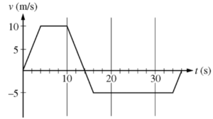
An object’s velocity \(v\) as a function of time \(t\) is given in the graph. Which of the following statements is true about the motion of the object?
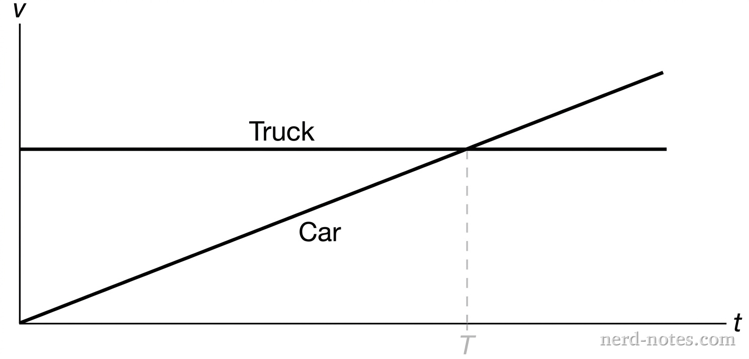
The motions of a car and a truck along a straight road are represented by the velocity–time graphs in the figure. The two vehicles are initially alongside each other at time \(t = 0\). At time \(T\), what is true of the distances traveled by the vehicles since time \(t = 0\)?
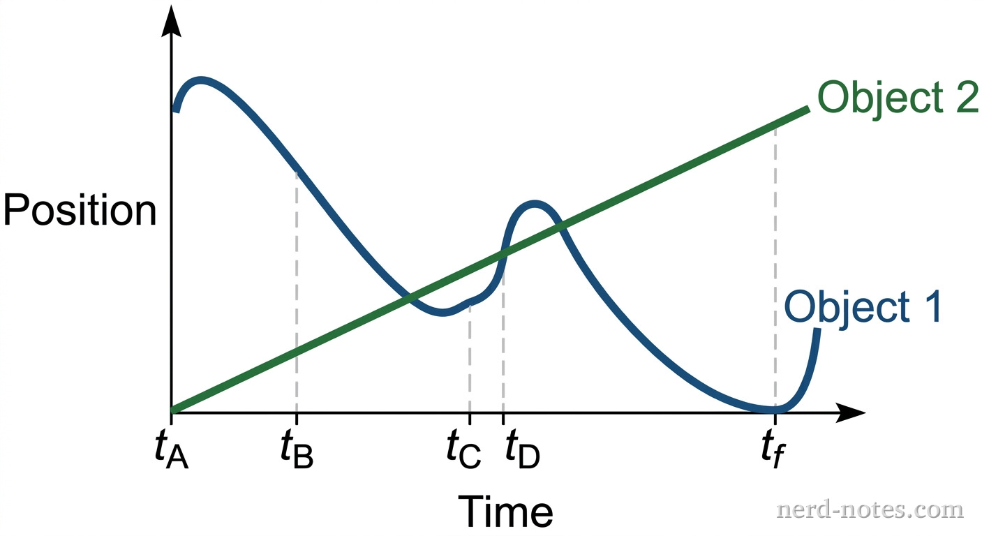
Which statement is true about the distances the two objects have traveled at time \( t_f \)?
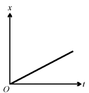
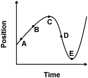
The displacement \( x \) of an object moving in one dimension is shown above as a function of time \( t \). The acceleration of this object must be
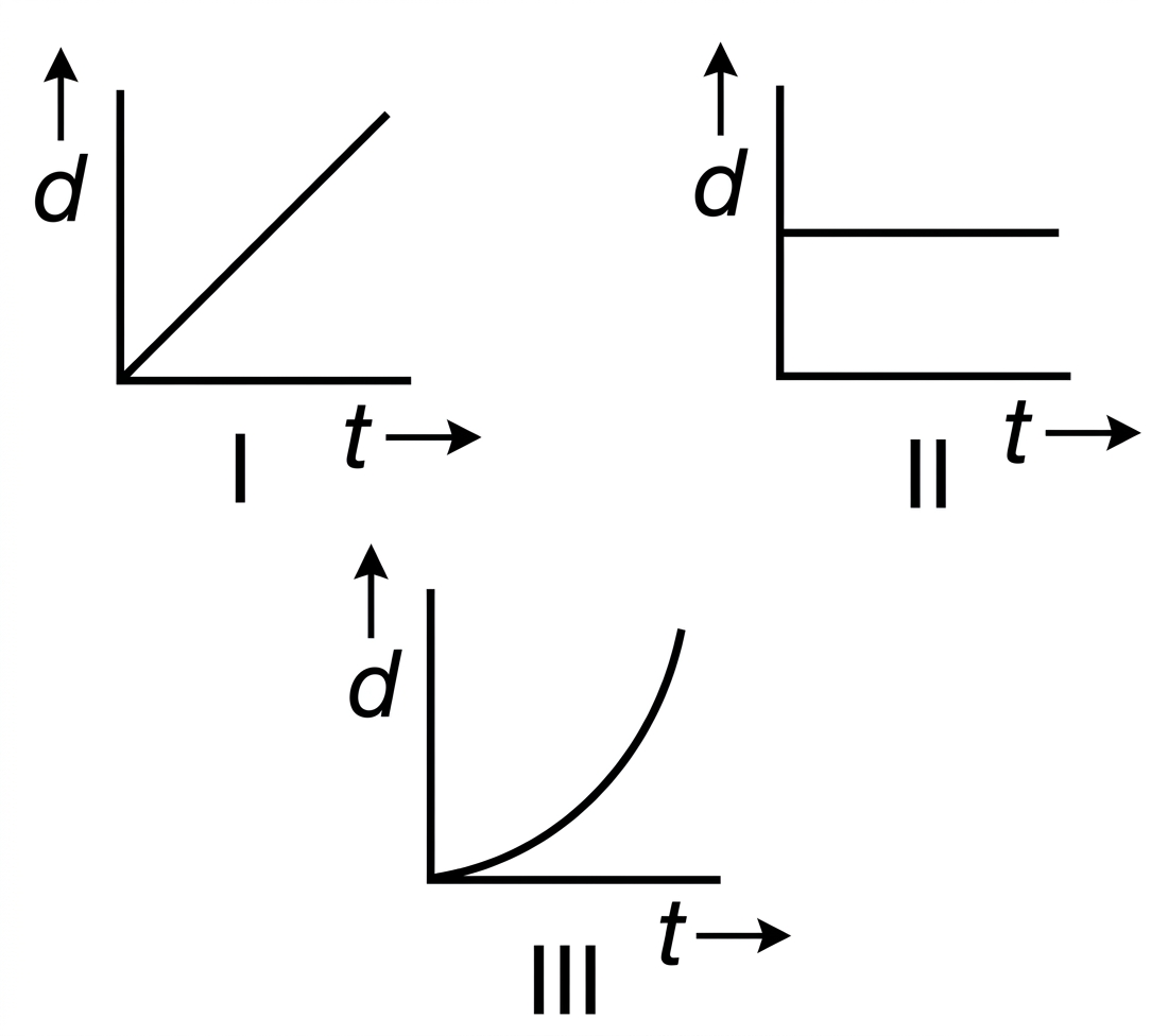 In which of the following is the particle’s acceleration constant?

A \( 0.20 \) \( \text{kg} \) object moves along a straight line. The net force acting on the object varies with the object’s displacement as shown in the graph above. The object starts from rest at displacement \( x = 0 \) and time \( t = 0 \) and is displaced a distance of \( 20 \) \( \text{m} \). Determine each of the following.
 Based on this graph…
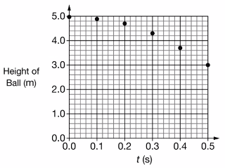
On another planet, a ball is in free fall after being released from rest at time \( t = 0 \). A graph of the height of the ball above the planet’s surface as a function of time \( t \) is shown. The acceleration due to gravity on the planet is most nearly


