
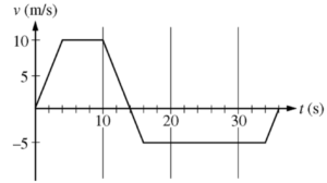
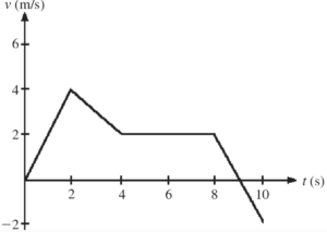
An object’s velocity \(v\) as a function of time \(t\) is given in the graph. Which of the following statements is true about the motion of the object?
A cart begins to move from rest on a horizontal track. Which of the following correctly indicates the magnitude of the average velocity of the cart during the interval shown and provides a valid explanation?
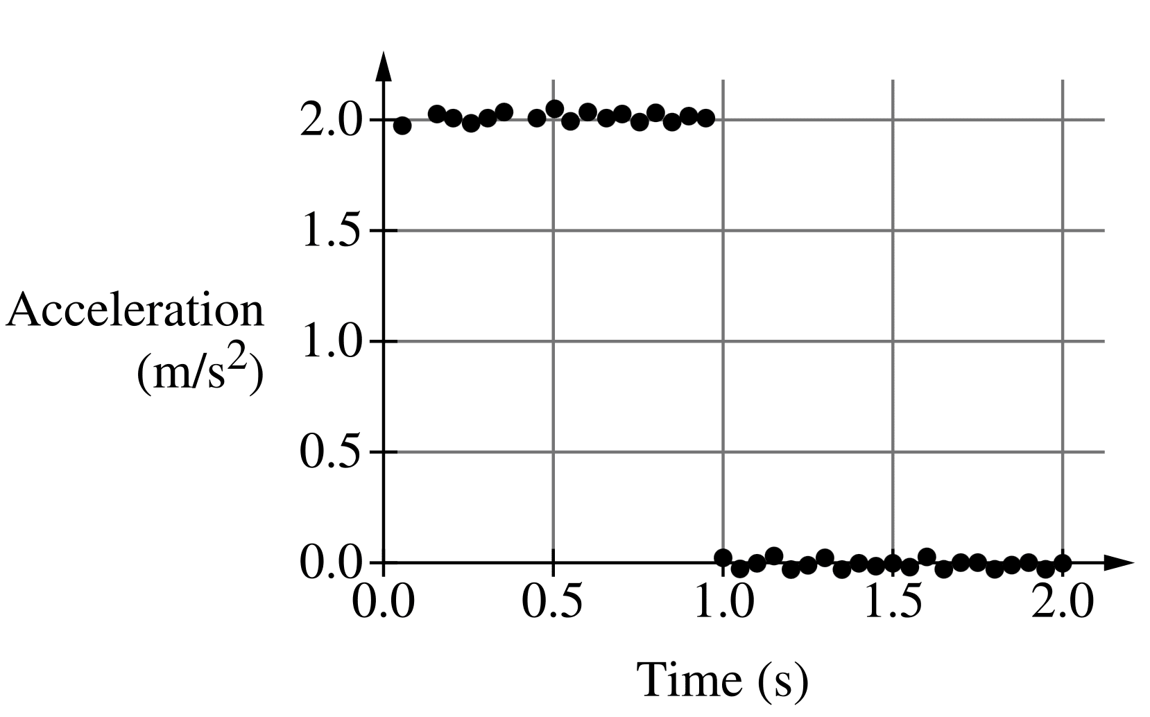
Hint: when solving this, its consider that the area of the acceleration vs time graph tells you the change in velocity.
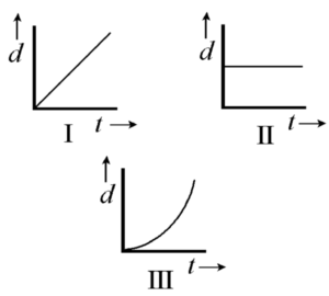
In which of the following is the rate of change of the particle’s momentum zero?
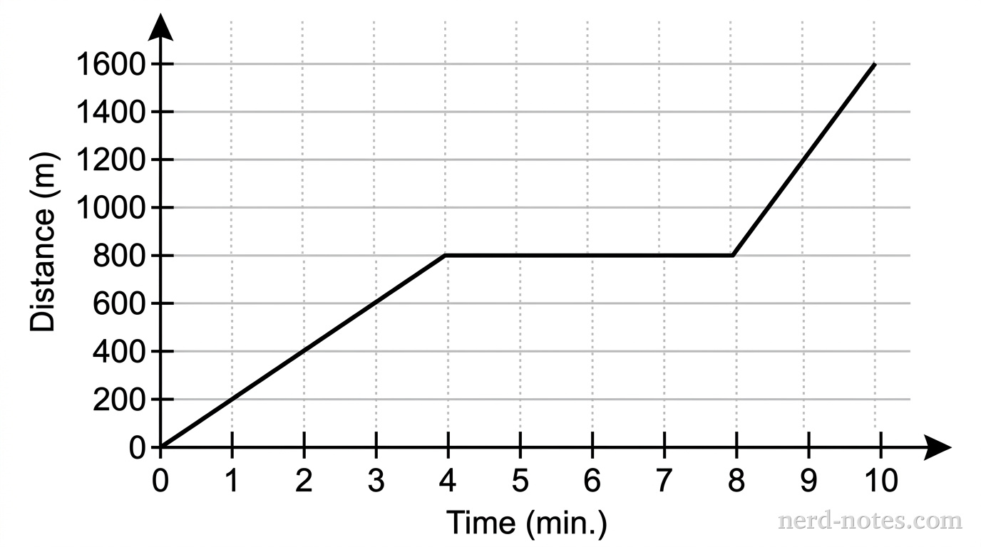
On Saturday, Ashley rode her bicycle to visit Maria. Maria’s house is directly east of Ashley’s. The graph shows how far Ashley was from her house after each minute of her trip. (Hint – Use the standard units of velocity \(\text{m/s}\) for all parts)
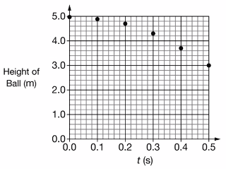
On another planet, a ball is in free fall after being released from rest at time \( t = 0 \). A graph of the height of the ball above the planet’s surface as a function of time \( t \) is shown. The acceleration due to gravity on the planet is most nearly
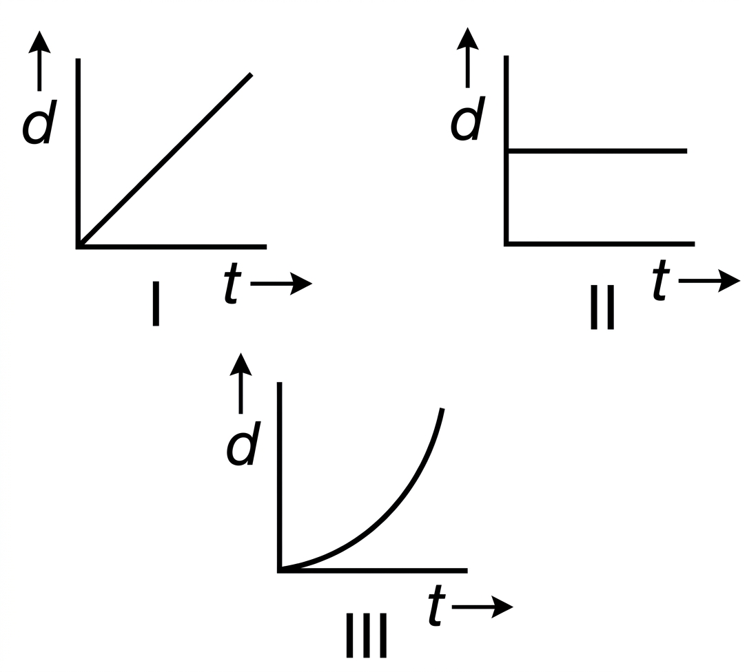 In which of the following is the particle’s acceleration constant?
The figure shows the velocity-versus-time graph for a basketball player traveling up and down the court in a straight-line path. Find the displacement of the player…
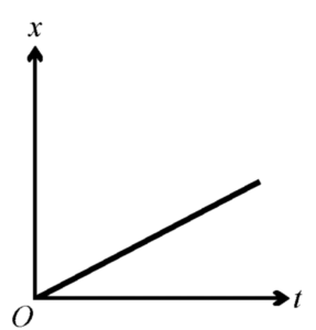
The displacement \( x \) of an object moving in one dimension is shown above as a function of time \( t \). The acceleration of this object must be


