| Step | Derivation/Formula | Reasoning |
|---|---|---|
| 1 | \[v=\frac{\Delta x}{\Delta t}\] | The velocity graph tells the slope of the position graph. When \(v\) is positive, \(x\) must increase; when \(v\) is negative, \(x\) must decrease; when \(v=0\), \(x\) has a local maximum or minimum. |
| 2 | \[v>0\Rightarrow x\text{ increases}\] | At the beginning, the velocity is positive and constant. Therefore, the position graph must initially rise with a constant positive slope. |
| 3 | \[v\text{ decreases from positive to negative}\] | In the middle interval, the velocity decreases smoothly through \(0\). Therefore, the slope of the position graph changes smoothly from positive to zero to negative. The position graph should reach a maximum when \(v=0\). |
| 4 | \[v<0\Rightarrow x\text{ decreases}\] | After the velocity crosses below zero, the position must decrease. Since the velocity eventually becomes a constant negative value, the position graph should end with a straight line of constant negative slope. |
| 5 | \[\boxed{\text{Choice A}}\] | Choice \(A\) shows position initially increasing, then reaching a maximum, then decreasing. This matches the sign change of velocity from positive to negative. Choices \(B\), \(C\), and \(D\) have flat or incorrect slope behavior, and choice \(E\) has sharp corners that imply sudden velocity changes not shown in the smooth velocity graph. |
A Major Upgrade To Phy Is Coming Soon — Stay Tuned

We'll help clarify entire units in one hour or less — guaranteed.
A self paced course with videos, problems sets, and everything you need to get a 5. Trusted by over 15k students and over 200 schools.
Can an object’s average velocity equal zero when object’s speed is greater than zero? Explain using the formula for average velocity vs speed.
A car travels east at a steady \( 30 \) \( \text{m/s} \) for \( 5 \) \( \text{s} \). What is its acceleration during this motion?
The first \(10 \, \text{meters}\) of a \(100 \, \text{meter}\) dash are covered in \(2 \, \text{seconds}\) by a sprinter who starts from rest and accelerates with a constant acceleration. The remaining \(90 \, \text{meters}\) are run with the same velocity the sprinter had after \(2 \, \text{seconds}\).
A car slows down uniformly from a speed of \( 28.0 \) \( \text{m/s} \) to rest in \( 8.00 \) \( \text{s} \). How far did it travel in that time?
You are a bungee jumping fanatic and want to be the first bungee jumper on Jupiter. The length of your bungee cord is \( 45.0 \) \( \text{m} \). Free fall acceleration on Jupiter is \( 23.1 \) \( \text{m/s}^2 \). What is the ratio of your speed on Jupiter to your speed on Earth when you have dropped \( 45 \) \( \text{m} \)? Ignore the effects of air resistance and assume that you start at rest.
A skater glides across the ice at a constant \( 6 \) \( \text{m/s} \). After \( 4 \) \( \text{s} \), friction gradually slows them down until they come to rest in \( 6 \) \( \text{s} \). They pause for \( 2 \) \( \text{s} \), then push off in the opposite direction, steadily gaining speed for \( 5 \) \( \text{s} \). Draw the velocity vs. time graph.
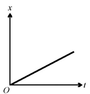 The displacement \(x\) of an object moving in one dimension is shown above as a function of time \(t\). The velocity of this object must be
A ball is dropped from a window \(10 \, \) above the sidewalk. Determine the time it takes for the ball to fall to the sidewalk.
A rollercoaster leaves the station at rest. Its speed increases steadily for \( 6 \) \( \text{s} \) as it heads down the first drop. The ride then levels out and it moves at a constant speed for \( 4 \) \( \text{s} \) before hitting the brakes and stopping in \( 3 \) \( \text{s} \). Draw the velocity vs. time graph or explain it in terms of functions.
Which pair of quantities will always have the same magnitude if motion is in a straight line and in one direction?
Graph A.
By continuing you (1) agree to our Terms of Use and Terms of Sale and (2) consent to sharing your IP and browser information used by this site’s security protocols as outlined in our Privacy Policy.
| Kinematics | Forces |
|---|---|
| \(\Delta x = v_i t + \frac{1}{2} at^2\) | \(F = ma\) |
| \(v = v_i + at\) | \(F_g = \frac{G m_1 m_2}{r^2}\) |
| \(v^2 = v_i^2 + 2a \Delta x\) | \(f = \mu N\) |
| \(\Delta x = \frac{v_i + v}{2} t\) | \(F_s =-kx\) |
| \(v^2 = v_f^2 \,-\, 2a \Delta x\) |
| Circular Motion | Energy |
|---|---|
| \(F_c = \frac{mv^2}{r}\) | \(KE = \frac{1}{2} mv^2\) |
| \(a_c = \frac{v^2}{r}\) | \(PE = mgh\) |
| \(T = 2\pi \sqrt{\frac{r}{g}}\) | \(KE_i + PE_i = KE_f + PE_f\) |
| \(W = Fd \cos\theta\) |
| Momentum | Torque and Rotations |
|---|---|
| \(p = mv\) | \(\tau = r \cdot F \cdot \sin(\theta)\) |
| \(J = \Delta p\) | \(I = \sum mr^2\) |
| \(p_i = p_f\) | \(L = I \cdot \omega\) |
| Simple Harmonic Motion | Fluids |
|---|---|
| \(F = -kx\) | \(P = \frac{F}{A}\) |
| \(T = 2\pi \sqrt{\frac{l}{g}}\) | \(P_{\text{total}} = P_{\text{atm}} + \rho gh\) |
| \(T = 2\pi \sqrt{\frac{m}{k}}\) | \(Q = Av\) |
| \(x(t) = A \cos(\omega t + \phi)\) | \(F_b = \rho V g\) |
| \(a = -\omega^2 x\) | \(A_1v_1 = A_2v_2\) |
| Constant | Description |
|---|---|
| [katex]g[/katex] | Acceleration due to gravity, typically [katex]9.8 , \text{m/s}^2[/katex] on Earth’s surface |
| [katex]G[/katex] | Universal Gravitational Constant, [katex]6.674 \times 10^{-11} , \text{N} \cdot \text{m}^2/\text{kg}^2[/katex] |
| [katex]\mu_k[/katex] and [katex]\mu_s[/katex] | Coefficients of kinetic ([katex]\mu_k[/katex]) and static ([katex]\mu_s[/katex]) friction, dimensionless. Static friction ([katex]\mu_s[/katex]) is usually greater than kinetic friction ([katex]\mu_k[/katex]) as it resists the start of motion. |
| [katex]k[/katex] | Spring constant, in [katex]\text{N/m}[/katex] |
| [katex] M_E = 5.972 \times 10^{24} , \text{kg} [/katex] | Mass of the Earth |
| [katex] M_M = 7.348 \times 10^{22} , \text{kg} [/katex] | Mass of the Moon |
| [katex] M_M = 1.989 \times 10^{30} , \text{kg} [/katex] | Mass of the Sun |
| Variable | SI Unit |
|---|---|
| [katex]s[/katex] (Displacement) | [katex]\text{meters (m)}[/katex] |
| [katex]v[/katex] (Velocity) | [katex]\text{meters per second (m/s)}[/katex] |
| [katex]a[/katex] (Acceleration) | [katex]\text{meters per second squared (m/s}^2\text{)}[/katex] |
| [katex]t[/katex] (Time) | [katex]\text{seconds (s)}[/katex] |
| [katex]m[/katex] (Mass) | [katex]\text{kilograms (kg)}[/katex] |
| Variable | Derived SI Unit |
|---|---|
| [katex]F[/katex] (Force) | [katex]\text{newtons (N)}[/katex] |
| [katex]E[/katex], [katex]PE[/katex], [katex]KE[/katex] (Energy, Potential Energy, Kinetic Energy) | [katex]\text{joules (J)}[/katex] |
| [katex]P[/katex] (Power) | [katex]\text{watts (W)}[/katex] |
| [katex]p[/katex] (Momentum) | [katex]\text{kilogram meters per second (kgm/s)}[/katex] |
| [katex]\omega[/katex] (Angular Velocity) | [katex]\text{radians per second (rad/s)}[/katex] |
| [katex]\tau[/katex] (Torque) | [katex]\text{newton meters (Nm)}[/katex] |
| [katex]I[/katex] (Moment of Inertia) | [katex]\text{kilogram meter squared (kgm}^2\text{)}[/katex] |
| [katex]f[/katex] (Frequency) | [katex]\text{hertz (Hz)}[/katex] |
Metric Prefixes
Example of using unit analysis: Convert 5 kilometers to millimeters.
Start with the given measurement: [katex]\text{5 km}[/katex]
Use the conversion factors for kilometers to meters and meters to millimeters: [katex]\text{5 km} \times \frac{10^3 \, \text{m}}{1 \, \text{km}} \times \frac{10^3 \, \text{mm}}{1 \, \text{m}}[/katex]
Perform the multiplication: [katex]\text{5 km} \times \frac{10^3 \, \text{m}}{1 \, \text{km}} \times \frac{10^3 \, \text{mm}}{1 \, \text{m}} = 5 \times 10^3 \times 10^3 \, \text{mm}[/katex]
Simplify to get the final answer: [katex]\boxed{5 \times 10^6 \, \text{mm}}[/katex]
Prefix | Symbol | Power of Ten | Equivalent |
|---|---|---|---|
Pico- | p | [katex]10^{-12}[/katex] | 0.000000000001 |
Nano- | n | [katex]10^{-9}[/katex] | 0.000000001 |
Micro- | µ | [katex]10^{-6}[/katex] | 0.000001 |
Milli- | m | [katex]10^{-3}[/katex] | 0.001 |
Centi- | c | [katex]10^{-2}[/katex] | 0.01 |
Deci- | d | [katex]10^{-1}[/katex] | 0.1 |
(Base unit) | – | [katex]10^{0}[/katex] | 1 |
Deca- or Deka- | da | [katex]10^{1}[/katex] | 10 |
Hecto- | h | [katex]10^{2}[/katex] | 100 |
Kilo- | k | [katex]10^{3}[/katex] | 1,000 |
Mega- | M | [katex]10^{6}[/katex] | 1,000,000 |
Giga- | G | [katex]10^{9}[/katex] | 1,000,000,000 |
Tera- | T | [katex]10^{12}[/katex] | 1,000,000,000,000 |
One price to unlock most advanced version of Phy across all our tools.
per month
Billed Monthly. Cancel Anytime.
Try our free calculator to see what you need to get a 5 on the 2026 AP Physics 1 exam.
A quick explanation
Credits are used to grade your FRQs and GQs. Pro users get unlimited credits.
Submitting counts as 1 attempt.
Viewing answers or explanations count as a failed attempts.
Phy gives partial credit if needed
MCQs and GQs are are 1 point each. FRQs will state points for each part.
Phy customizes problem explanations based on what you struggle with. Just hit the explanation button to see.
Understand you mistakes quicker.

Phy automatically provides feedback so you can improve your responses.
10 Free Credits To Get You Started

By continuing you agree to nerd-notes.com Terms of Service, Privacy Policy, and our usage of user data.
Feeling uneasy about your next physics test? We'll boost your grade in 3 lessons or less—guaranteed

NEW! PHY AI accurately solves all questions
🔥 Get up to 30% off Elite Physics Tutoring
🧠 NEW! Learn Physics From Scratch Self Paced Course
🎯 Need exam style practice questions?
