
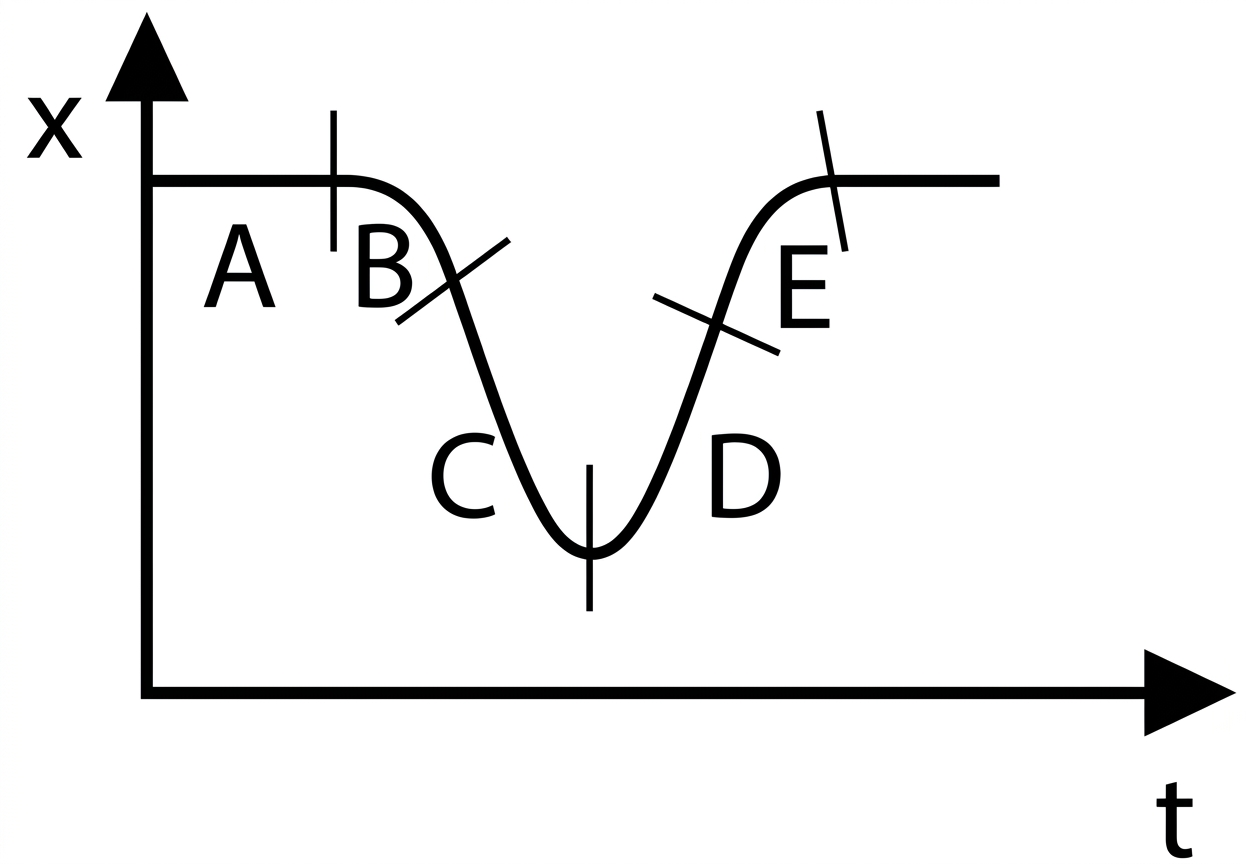
 The graph below is a plot of position versus time. For which labeled segments is the velocity positive and the acceleration negative?

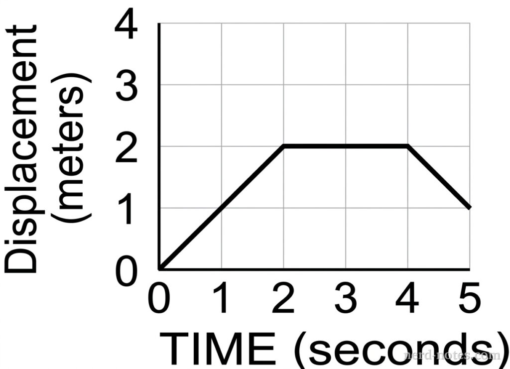
The graph above represents the motion of an object traveling in a straight line as a function of time. What is the average speed of the object during the first four seconds?
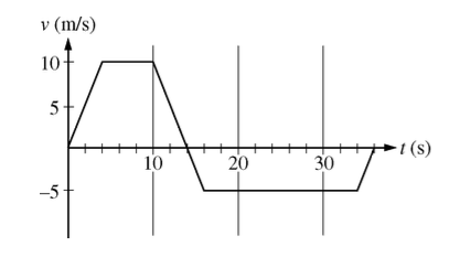
Above is the graph of an object’s velocity as a function of time. Which of the following is true about the motion?
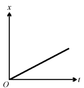
The displacement \( x \) of an object moving in one dimension is shown above as a function of time \( t \). The acceleration of this object must be
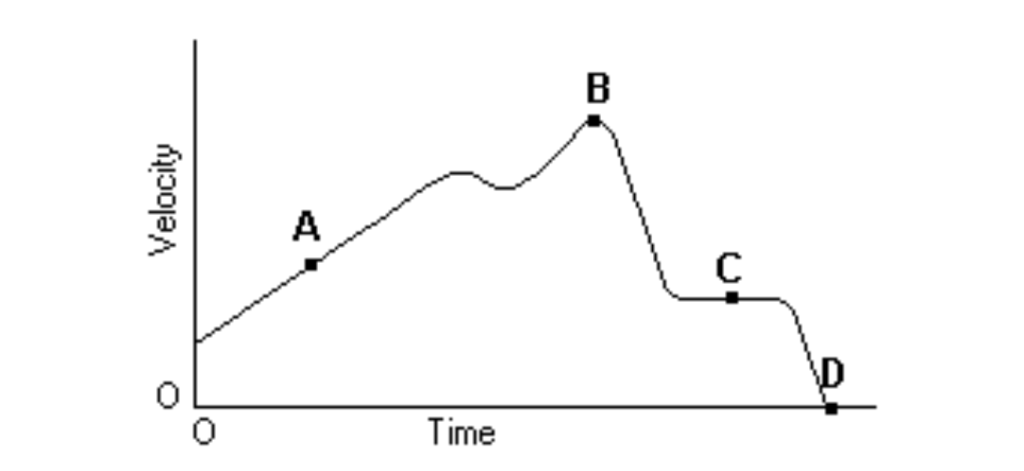 Above is the graph of the velocity vs. time of a duck flying due south for the winter. At what point might the duck begin reversing directions?
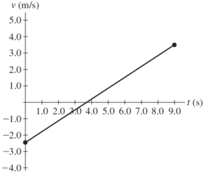
The motion of a particle is described in the velocity vs. time graph shown above. Over the nine-second interval shown, we can say that the speed of the particle…
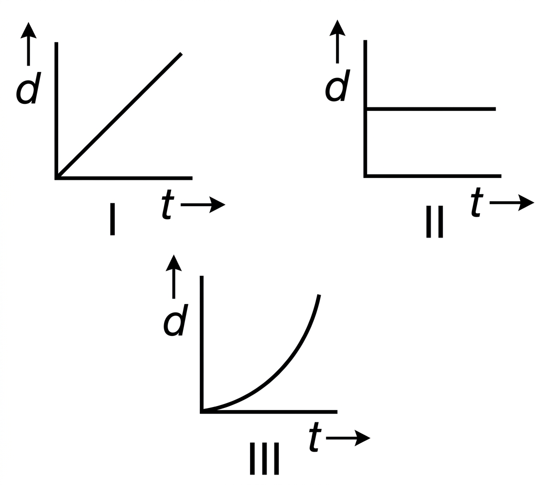 In which of the following is the particle’s acceleration constant?
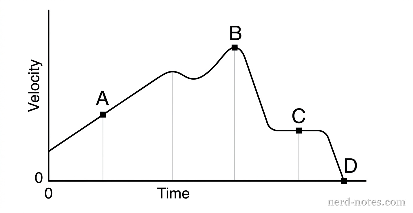
Given the graph of velocity versus time for a duck flying due south for the winter, at what labeled point did the duck stop its forward motion?


