
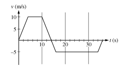
Above is the graph of an object’s velocity as a function of time. Which of the following is true about the motion?
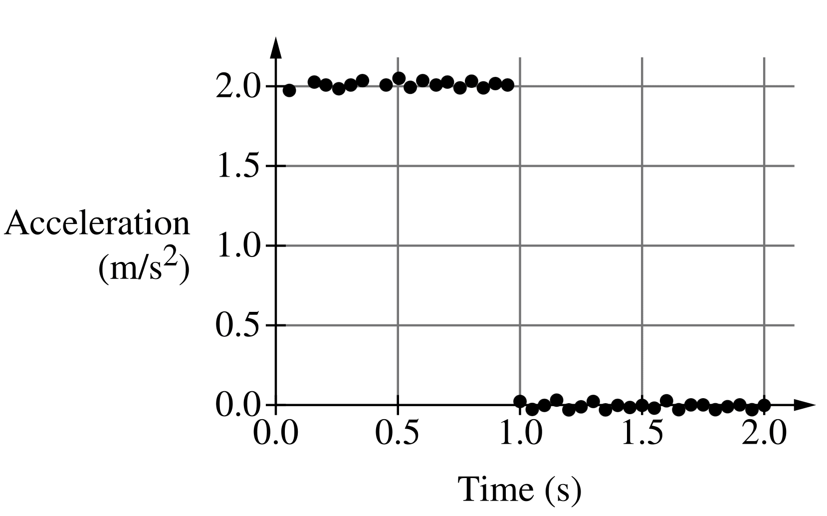
The graph shows the acceleration as a function of time for an object that is at rest at time \( t = 0 \) \( \text{s} \). The distance traveled by the object between \( 0 \) and \( 2 \) \( \text{s} \) is most nearly
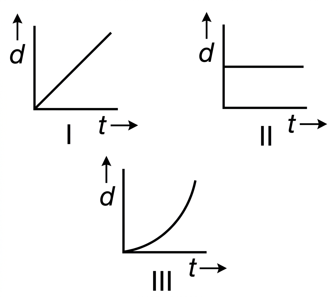 In which of the following is the particle’s acceleration constant?
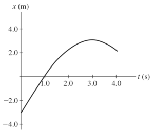
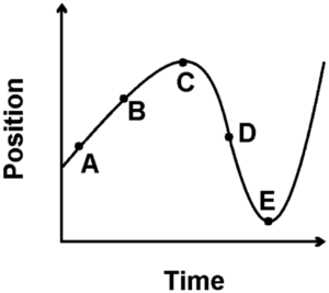
The graph in the figure shows the position of a particle as it travels along the x-axis. At what value of \(t\) is the speed of the particle equal to \(0 \, \text{m/s}\)?
note that the slope of position vs time is velocity. And the graph most closely reemsbles a flat or 0 slope at 3 seconds
A cart begins to move from rest on a horizontal track. Which of the following correctly indicates the magnitude of the average velocity of the cart during the interval shown and provides a valid explanation?
Hint: when solving this, its consider that the area of the acceleration vs time graph tells you the change in velocity.
 Based on this graph…
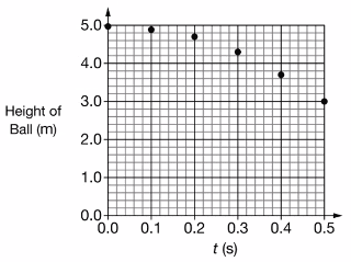
On another planet, a ball is in free fall after being released from rest at time \( t = 0 \). A graph of the height of the ball above the planet’s surface as a function of time \( t \) is shown. The acceleration due to gravity on the planet is most nearly


