| Derivation / Formula | Reasoning |
|---|---|
| \[x(t)=A\cos\left(\frac{2\pi t}{T}\right)\] | The cosine form matches the graph: at \(t=0\) the displacement is \(+A\). |
| \[v(t)=\frac{dx}{dt}=-A\left(\frac{2\pi}{T}\right)\sin\left(\frac{2\pi t}{T}\right)\] | Velocity is the time–derivative of displacement. Its sign depends on \(\sin\left(\frac{2\pi t}{T}\right)\). |
| \[a(t)=\frac{dv}{dt}=-\left(\frac{2\pi}{T}\right)^{2}A\cos\left(\frac{2\pi t}{T}\right)\] | Acceleration is the derivative of velocity or \(-\omega^{2}x\), always directed toward equilibrium. |
| \[x\!\left(\frac{T}{2}\right)=A\cos\pi=-A\] | Half a period after the start, the bob is at the negative extreme. |
| \[v\!\left(\frac{T}{2}\right)=-A\left(\frac{2\pi}{T}\right)\sin\pi=0\] | At the turning point the bob instantaneously stops before reversing, so velocity is zero. |
| \[a\!\left(\frac{T}{2}\right)=-\left(\frac{2\pi}{T}\right)^{2}A\cos\pi=+\left(\frac{2\pi}{T}\right)^{2}A>0\] | Because \(x\) is negative, the restoring acceleration points toward the positive equilibrium position, giving a positive value. |
| \[\boxed{v=0,\;a>0}\] | This corresponds to choice (D). |
| — | (A) & (C): Velocity would indeed be negative while moving downward, but at \(t=\frac{T}{2}\) the bob has already stopped, so \(v<0\) is wrong. Acceleration signs given are also inconsistent with the restoring direction. |
| — | (B): Claims \(v<0\) though velocity is actually zero at the extreme; further, acceleration is not zero at an extreme position. |
| — | (E): Both velocity and acceleration cannot be zero simultaneously for simple harmonic motion unless the bob is at equilibrium with no motion, which is not the case here. |
A Major Upgrade To Phy Is Coming Soon — Stay Tuned

We'll help clarify entire units in one hour or less — guaranteed.
A self paced course with videos, problems sets, and everything you need to get a 5. Trusted by over 15k students and over 200 schools.
A student uses a pendulum to determine the acceleration due to gravity, \( g \). They measure the pendulum’s length \( L \) and its period \( T \). Which equation should they use to calculate \( g \)?
A \( 2 \, \text{kg}\) mass is attached to a spring with spring constant \( k = 100 \, \text{N/m}\) and negligible mass.
A block attached to spring demonstrates simple harmonic motion about its equilibrium position with amplitude \( A \) and angular frequency \( \omega \). What is the maximum magnitude of the block’s velocity?
A student is designing an experiment to find the spring constant \( k \) of a spring using only a set of known masses and a stopwatch. Which procedure would work?
A mass–spring system is oscillating in simple harmonic motion. At the exact moment the mass passes through its equilibrium position, which of the following statements is true?
An average adult elephant \( (5000 \, \text{kg}) \) is strapped to a spring, which is then pulled \( 2 \, \text{meters} \) away from its equilibrium position and released. The elephant starts oscillating back and forth with a period of \( 10 \) seconds.
A Christmas ornament made from a thin hollow glass sphere hangs from a thin wire of negligible mass. It is observed to oscillates with a frequency of \( 2.50 \) \( \text{Hz} \) in a city where \( g = 9.80 \) \( \text{m/s}^2 \). What is the radius of the ornament? The moment of inertia of the ornament is given by \( I = \frac{5}{3} mr^2 \).
What is the effect on the period of a pendulum if you double its length?
A box of mass \( 20 \) \( \text{kg} \) moves to the right on a horizontal frictionless surface with a speed of \( 4.0 \) \( \text{m/s} \). The box collides with and remains attached to one end of a spring of negligible mass whose other end is fixed to a wall. After the collision, the spring compresses a maximum distance of \( 0.50 \) \( \text{m} \), and the box then oscillates back and forth.
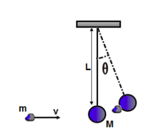
A \(20 \, \text{g}\) piece of clay moving at a speed of \(50 \, \text{m/s}\) strikes a \(500 \, \text{g}\) pendulum bob at rest. The length of a string is \(0.8 \, \text{m}\). After the collision, the clay-bob system starts to oscillate as a simple pendulum.
By continuing you (1) agree to our Terms of Use and Terms of Sale and (2) consent to sharing your IP and browser information used by this site’s security protocols as outlined in our Privacy Policy.
| Kinematics | Forces |
|---|---|
| \(\Delta x = v_i t + \frac{1}{2} at^2\) | \(F = ma\) |
| \(v = v_i + at\) | \(F_g = \frac{G m_1 m_2}{r^2}\) |
| \(v^2 = v_i^2 + 2a \Delta x\) | \(f = \mu N\) |
| \(\Delta x = \frac{v_i + v}{2} t\) | \(F_s =-kx\) |
| \(v^2 = v_f^2 \,-\, 2a \Delta x\) |
| Circular Motion | Energy |
|---|---|
| \(F_c = \frac{mv^2}{r}\) | \(KE = \frac{1}{2} mv^2\) |
| \(a_c = \frac{v^2}{r}\) | \(PE = mgh\) |
| \(T = 2\pi \sqrt{\frac{r}{g}}\) | \(KE_i + PE_i = KE_f + PE_f\) |
| \(W = Fd \cos\theta\) |
| Momentum | Torque and Rotations |
|---|---|
| \(p = mv\) | \(\tau = r \cdot F \cdot \sin(\theta)\) |
| \(J = \Delta p\) | \(I = \sum mr^2\) |
| \(p_i = p_f\) | \(L = I \cdot \omega\) |
| Simple Harmonic Motion | Fluids |
|---|---|
| \(F = -kx\) | \(P = \frac{F}{A}\) |
| \(T = 2\pi \sqrt{\frac{l}{g}}\) | \(P_{\text{total}} = P_{\text{atm}} + \rho gh\) |
| \(T = 2\pi \sqrt{\frac{m}{k}}\) | \(Q = Av\) |
| \(x(t) = A \cos(\omega t + \phi)\) | \(F_b = \rho V g\) |
| \(a = -\omega^2 x\) | \(A_1v_1 = A_2v_2\) |
| Constant | Description |
|---|---|
| [katex]g[/katex] | Acceleration due to gravity, typically [katex]9.8 , \text{m/s}^2[/katex] on Earth’s surface |
| [katex]G[/katex] | Universal Gravitational Constant, [katex]6.674 \times 10^{-11} , \text{N} \cdot \text{m}^2/\text{kg}^2[/katex] |
| [katex]\mu_k[/katex] and [katex]\mu_s[/katex] | Coefficients of kinetic ([katex]\mu_k[/katex]) and static ([katex]\mu_s[/katex]) friction, dimensionless. Static friction ([katex]\mu_s[/katex]) is usually greater than kinetic friction ([katex]\mu_k[/katex]) as it resists the start of motion. |
| [katex]k[/katex] | Spring constant, in [katex]\text{N/m}[/katex] |
| [katex] M_E = 5.972 \times 10^{24} , \text{kg} [/katex] | Mass of the Earth |
| [katex] M_M = 7.348 \times 10^{22} , \text{kg} [/katex] | Mass of the Moon |
| [katex] M_M = 1.989 \times 10^{30} , \text{kg} [/katex] | Mass of the Sun |
| Variable | SI Unit |
|---|---|
| [katex]s[/katex] (Displacement) | [katex]\text{meters (m)}[/katex] |
| [katex]v[/katex] (Velocity) | [katex]\text{meters per second (m/s)}[/katex] |
| [katex]a[/katex] (Acceleration) | [katex]\text{meters per second squared (m/s}^2\text{)}[/katex] |
| [katex]t[/katex] (Time) | [katex]\text{seconds (s)}[/katex] |
| [katex]m[/katex] (Mass) | [katex]\text{kilograms (kg)}[/katex] |
| Variable | Derived SI Unit |
|---|---|
| [katex]F[/katex] (Force) | [katex]\text{newtons (N)}[/katex] |
| [katex]E[/katex], [katex]PE[/katex], [katex]KE[/katex] (Energy, Potential Energy, Kinetic Energy) | [katex]\text{joules (J)}[/katex] |
| [katex]P[/katex] (Power) | [katex]\text{watts (W)}[/katex] |
| [katex]p[/katex] (Momentum) | [katex]\text{kilogram meters per second (kgm/s)}[/katex] |
| [katex]\omega[/katex] (Angular Velocity) | [katex]\text{radians per second (rad/s)}[/katex] |
| [katex]\tau[/katex] (Torque) | [katex]\text{newton meters (Nm)}[/katex] |
| [katex]I[/katex] (Moment of Inertia) | [katex]\text{kilogram meter squared (kgm}^2\text{)}[/katex] |
| [katex]f[/katex] (Frequency) | [katex]\text{hertz (Hz)}[/katex] |
Metric Prefixes
Example of using unit analysis: Convert 5 kilometers to millimeters.
Start with the given measurement: [katex]\text{5 km}[/katex]
Use the conversion factors for kilometers to meters and meters to millimeters: [katex]\text{5 km} \times \frac{10^3 \, \text{m}}{1 \, \text{km}} \times \frac{10^3 \, \text{mm}}{1 \, \text{m}}[/katex]
Perform the multiplication: [katex]\text{5 km} \times \frac{10^3 \, \text{m}}{1 \, \text{km}} \times \frac{10^3 \, \text{mm}}{1 \, \text{m}} = 5 \times 10^3 \times 10^3 \, \text{mm}[/katex]
Simplify to get the final answer: [katex]\boxed{5 \times 10^6 \, \text{mm}}[/katex]
Prefix | Symbol | Power of Ten | Equivalent |
|---|---|---|---|
Pico- | p | [katex]10^{-12}[/katex] | 0.000000000001 |
Nano- | n | [katex]10^{-9}[/katex] | 0.000000001 |
Micro- | µ | [katex]10^{-6}[/katex] | 0.000001 |
Milli- | m | [katex]10^{-3}[/katex] | 0.001 |
Centi- | c | [katex]10^{-2}[/katex] | 0.01 |
Deci- | d | [katex]10^{-1}[/katex] | 0.1 |
(Base unit) | – | [katex]10^{0}[/katex] | 1 |
Deca- or Deka- | da | [katex]10^{1}[/katex] | 10 |
Hecto- | h | [katex]10^{2}[/katex] | 100 |
Kilo- | k | [katex]10^{3}[/katex] | 1,000 |
Mega- | M | [katex]10^{6}[/katex] | 1,000,000 |
Giga- | G | [katex]10^{9}[/katex] | 1,000,000,000 |
Tera- | T | [katex]10^{12}[/katex] | 1,000,000,000,000 |
One price to unlock most advanced version of Phy across all our tools.
per month
Billed Monthly. Cancel Anytime.
Try our free calculator to see what you need to get a 5 on the 2026 AP Physics 1 exam.
A quick explanation
Credits are used to grade your FRQs and GQs. Pro users get unlimited credits.
Submitting counts as 1 attempt.
Viewing answers or explanations count as a failed attempts.
Phy gives partial credit if needed
MCQs and GQs are are 1 point each. FRQs will state points for each part.
Phy customizes problem explanations based on what you struggle with. Just hit the explanation button to see.
Understand you mistakes quicker.

Phy automatically provides feedback so you can improve your responses.
10 Free Credits To Get You Started

By continuing you agree to nerd-notes.com Terms of Service, Privacy Policy, and our usage of user data.
Feeling uneasy about your next physics test? We'll boost your grade in 3 lessons or less—guaranteed

NEW! PHY AI accurately solves all questions
🔥 Get up to 30% off Elite Physics Tutoring
🧠 NEW! Learn Physics From Scratch Self Paced Course
🎯 Need exam style practice questions?
