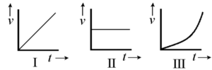
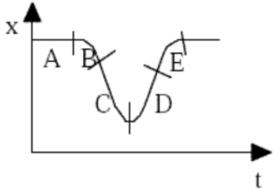
In which of the following is the rate of change of the particle’s momentum zero?

A \( 0.20 \) \( \text{kg} \) object moves along a straight line. The net force acting on the object varies with the object’s displacement as shown in the graph above. The object starts from rest at displacement \( x = 0 \) and time \( t = 0 \) and is displaced a distance of \( 20 \) \( \text{m} \). Determine each of the following.
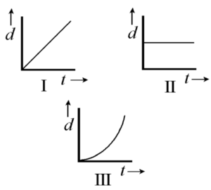
In which of these cases is the rate of change of the particle’s displacement constant?
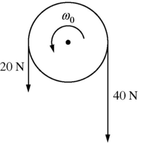
A disk is initially rotating counterclockwise around a fixed axis with angular speed \( \omega_0 \). At time \( t = 0 \), the two forces shown in the figure above are exerted on the disk. If counterclockwise is positive, which of the following could show the angular velocity of the disk as a function of time?
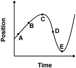
 The graph below is a plot of position versus time. For which labeled segments is the velocity positive and the acceleration negative?
 Based on this graph…
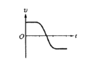
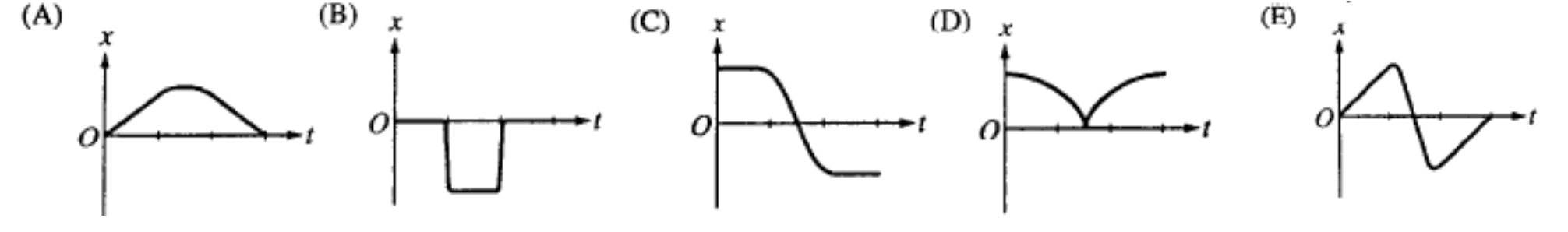
The graph above shows velocity \( v \) versus time \( t \) for an object in linear motion. Which of the following is a possible graph of position (\( x \)) versus time (\( t \)) for this object?