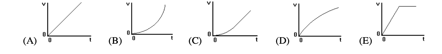
A large beach ball is dropped from the ceiling of a school gymnasium to the floor about 10 meters below. Which of the following graphs would best represent its velocity as a function of time? (do not neglect air resistance)
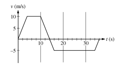
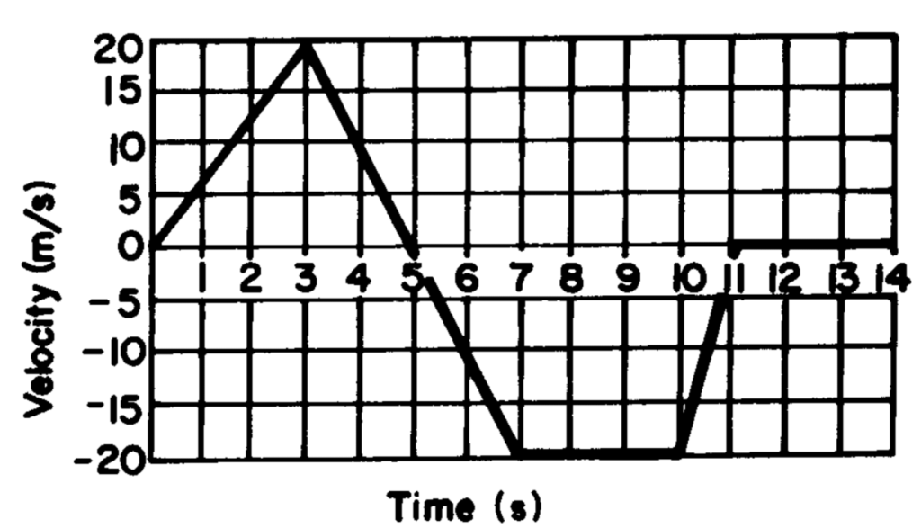
Above is the graph of an object’s velocity as a function of time. Which of the following is true about the motion?
 Based on this graph…
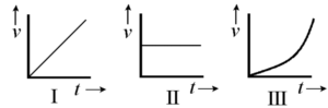
In which of these cases is the rate of change of the particle’s displacement constant?

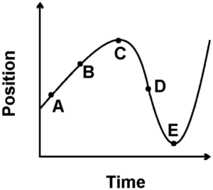
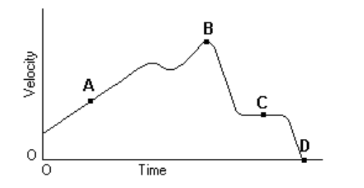 Given the graph of velocity versus time for a duck flying due south for the winter, at what labeled point did the duck stop its forward motion?


