
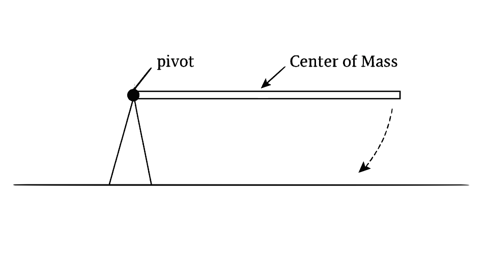
A uniform rod of length \( L \) and mass \( M \) is free to rotate about one end, as shown in the diagram. The free end is released from rest at a horizontal position, as shown. The pivot point is supported by a stand so that only the free end can move. The moment of inertia of a rod about its end is \(\tfrac{1}{3} M L^{2}\).
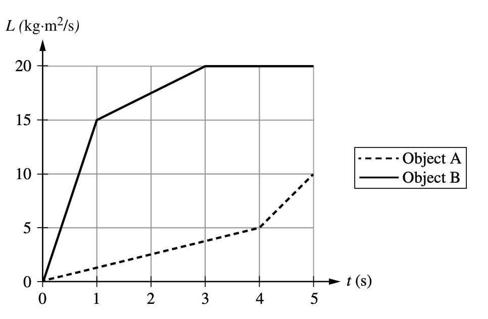
Two disks, A and B, each experience a net external torque that varies over an interval of \( 5 \) \( \text{s} \). Disk B has a rotational inertia that is twice that of Disk A. The graph shown represents the angular momentum of the two disks as functions of time between \( t = 0 \) \( \text{s} \) and \( t = 5 \) \( \text{s} \). The average magnitudes of the net torques exerted on disks A and B from \( t = 0 \) \( \text{s} \) to \( t = 5 \) \( \text{s} \) are \( \tau_A \) and \( \tau_B \), respectively. Which of the following expressions correctly relates the magnitudes of the average torques?

A meter stick with a uniformly distributed mass of \(0.5 \, \text{kg}\) is supported by a pivot placed at the \(0.25 \, \text{m}\) mark from the left. At the left end, a small object of mass \(1.0 \, \text{kg}\) is placed at the zero mark, and a second small object of mass \(0.5 \, \text{kg}\) is placed at the \(0.5 \, \text{m}\) mark. The meter stick is supported so that it remains horizontal, and then it is released from rest. Find the change in the angular momentum of the meter stick, one second after it is released.
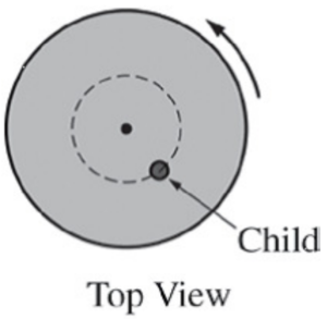
The diagram above shows a top view of a child of mass \(M\) on a circular platform of mass \(2M\) that is rotating counterclockwise. Assume the platform rotates without friction. Which of the following describes an action by the child that will increase the angular speed of the platform-child system and gives the correct reason why?


