
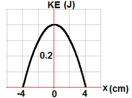
A 0.2 kg object is attached to a horizontal spring undergoes SHM with the total energy of 0.4 J. The kinetic energy as a function of position presented by the graph.
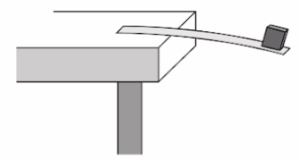
Students attach a thin strip of metal to a table so that the strip is horizontal in relation to the ground. A section of the strip hangs off the edge of the table. A mass is secured to the end of the hanging section of the strip and is then displaced so that the mass-strip system oscillates, as shown in the figure. Students make various measurements of the net force \( F \) exerted on the mass as a result of the force due to gravity and the normal force from the strip, the vertical position \( y \) of the mass above and below its equilibrium position \( y \), and the period of oscillation \( T’ \) when the mass is displaced by different amplitudes \( A \). Which of the following explanations is correct about the evidence required to conclude that the mass undergoes simple harmonic motion?
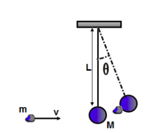
A \(20 \, \text{g}\) piece of clay moving at a speed of \(50 \, \text{m/s}\) strikes a \(500 \, \text{g}\) pendulum bob at rest. The length of a string is \(0.8 \, \text{m}\). After the collision, the clay-bob system starts to oscillate as a simple pendulum.

A simple pendulum consists of a bob of mass 1.8 kg attached to a string of length 2.3 m. The pendulum is held at an angle of 30° from the vertical by a light horizontal string attached to a wall, as shown above.

The graph represents the position \( x \) as a function of time \( t \) for an object undergoing simple harmonic motion. Which of the following equations could represent the position \( x \) as a function of time \( t \)?


