Part (a) – Finding the Average Speed
| Step | Derivation/Formula | Reasoning |
|---|---|---|
| 1 | \( v_{\text{initial}} = 20 \, \text{m/s} \) | The initial speed of the car is given as \( 20 \, \text{m/s} \). |
| 2 | \( v_{\text{final}} = 0 \, \text{m/s} \) | The car comes to a complete stop, so the final speed is \( 0 \, \text{m/s} \). |
| 3 | \( v_{\text{avg}} = \frac{v_{\text{initial}} + v_{\text{final}}}{2} \) | The average speed is the arithmetic mean of the initial and final speeds. |
| 4 | \( v_{\text{avg}} = \frac{20 \, \text{m/s} + 0 \, \text{m/s}}{2} = 10 \, \text{m/s} \) | Calculating the average speed. The average speed of the car is \( 10 \, \text{m/s} \). |
Part (b) – Determining the Time to Stop
| Step | Derivation/Formula | Reasoning |
|---|---|---|
| 1 | \( d = 40 \, \text{m} \) | The car travels \( 40 \, \text{m} \) before coming to a stop. |
| 2 | \( t = \frac{d}{v_{\text{avg}}} \) | Time can be found using the formula for distance, \( d = v_{\text{avg}} \cdot t \), rearranged to solve for \( t \). |
| 3 | \( t = \frac{40 \, \text{m}}{10 \, \text{m/s}} = 4 \, \text{s} \) | Substituting the values of distance and average speed to calculate the time. It takes \( 4 \, \text{s} \) for the car to stop. |
A Major Upgrade To Phy Is Coming Soon — Stay Tuned

We'll help clarify entire units in one hour or less — guaranteed.
A self paced course with videos, problems sets, and everything you need to get a 5. Trusted by over 15k students and over 200 schools.
You are standing on a bathroom scale in an elevator. The elevator starts from rest on the first floor and accelerates up to the third floor, \(12 \, \text{m}\) above, in a time of \(6 \, \text{s}\). The scale reads \(800 \, \text{N}\). What is the mass of the person?
A skateboarder, with an initial speed of \( 20.0 \, \text{m/s} \), rolls to the end of friction-free incline of length \( 25 \, \text{m} \). At what angle is the incline oriented above the horizontal?
Priscilla the Penguin stands at the edge of a rock ledge and tosses a small ice cube directly upward with an initial velocity of \( v_0 \). The ice cube’s initial height above the ground is \( 3.25 \, \text{m} \), and it reaches its maximum height above the ground \( 0.586 \, \text{s} \) after being thrown. The ice cube then plummets to the ground, missing the edge of the rock ledge on its way down.
An object is thrown downward at \(23 ~\text{m/s}\) from the top of a \(200 ~\text{m}\) tall building.
Does the odometer of a car measure a scalar or a vector quantity? What about the speedometer?
Which pair of quantities will always have the same magnitude if motion is in a straight line and in one direction?
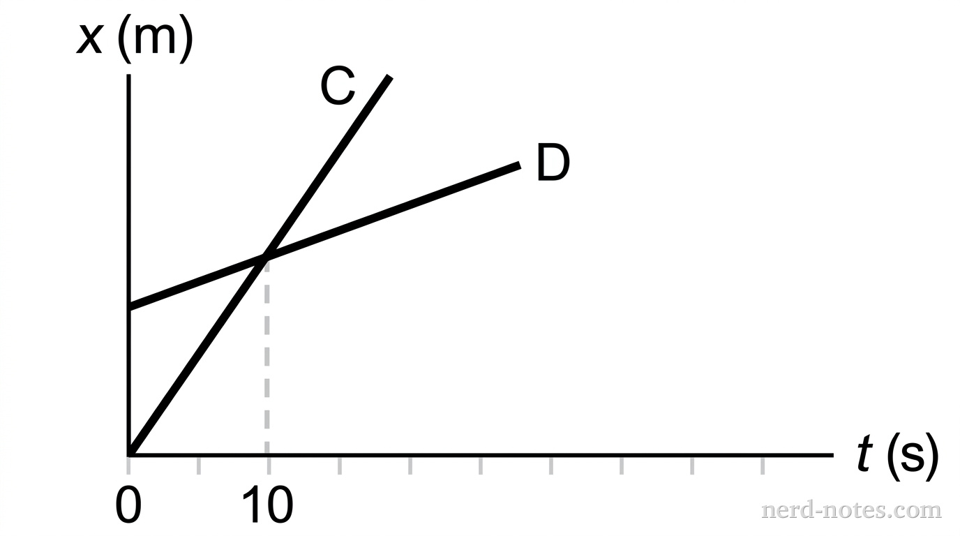
The figure shows a graph of the position \(x\) of two cars, \(C\) and \(D\), as a function of time \(t\). According to this graph, which statements about these cars must be true? (There could be more than one correct choice.)
A car is driving to the right at \( 20 \) \( \text{m/s} \). A motorcycle starts \( 30 \) \( \text{m} \) behind the car and is moving at \( 30 \) \( \text{m/s} \) in the same direction.
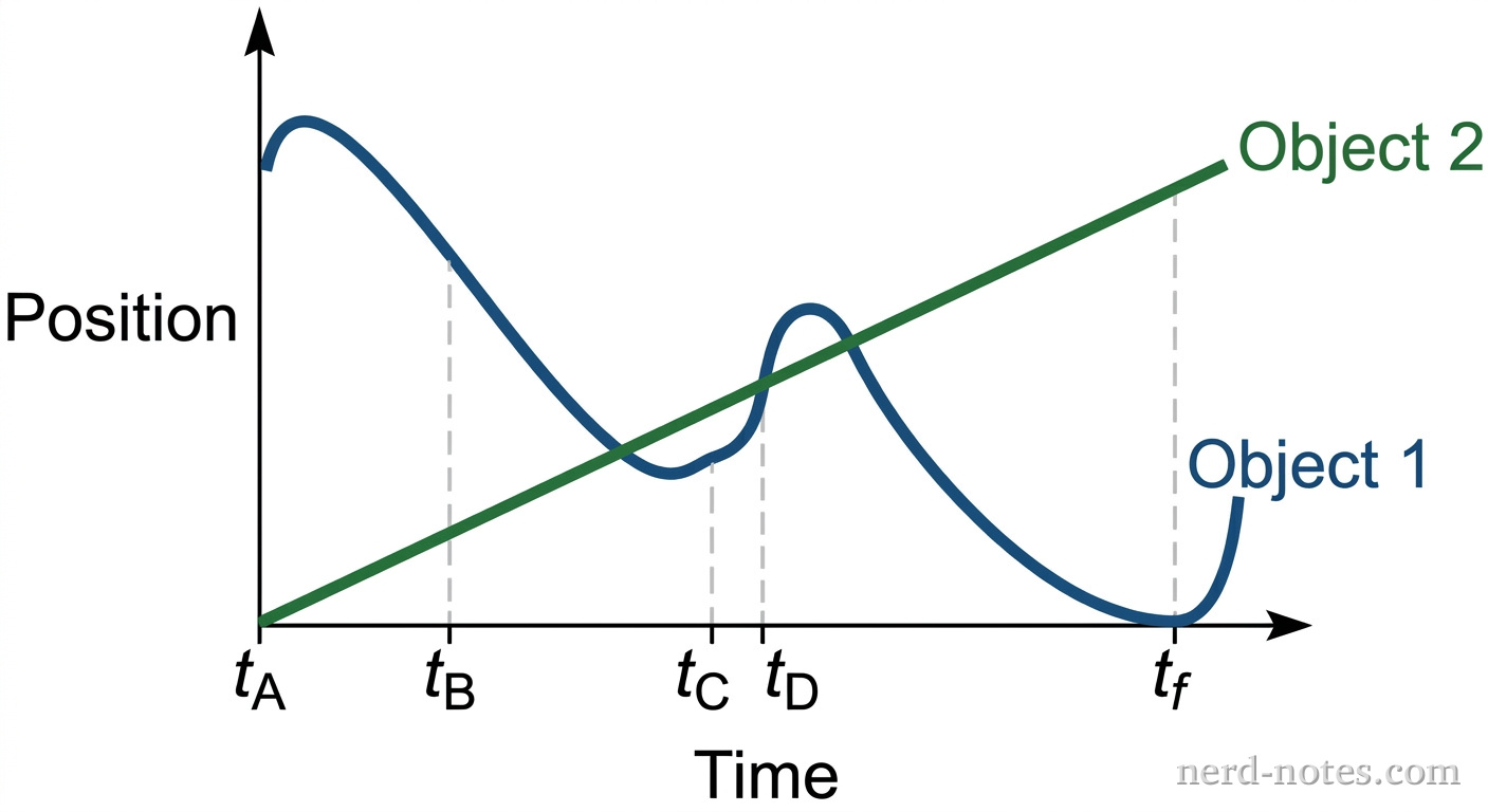
Which statement is true about the distances the two objects have traveled at time \( t_f \)?
An elevator of height \(h\) ascends with constant acceleration \(a\). When it crosses a platform, it has acquired a velocity \(u\). At this instant a bolt drops from the top of the elevator. Find the time for the bolt to hit the floor of the elevator. Give your answer in terms of \(h\), \(a\), and any constant.
By continuing you (1) agree to our Terms of Use and Terms of Sale and (2) consent to sharing your IP and browser information used by this site’s security protocols as outlined in our Privacy Policy.
| Kinematics | Forces |
|---|---|
| \(\Delta x = v_i t + \frac{1}{2} at^2\) | \(F = ma\) |
| \(v = v_i + at\) | \(F_g = \frac{G m_1 m_2}{r^2}\) |
| \(v^2 = v_i^2 + 2a \Delta x\) | \(f = \mu N\) |
| \(\Delta x = \frac{v_i + v}{2} t\) | \(F_s =-kx\) |
| \(v^2 = v_f^2 \,-\, 2a \Delta x\) |
| Circular Motion | Energy |
|---|---|
| \(F_c = \frac{mv^2}{r}\) | \(KE = \frac{1}{2} mv^2\) |
| \(a_c = \frac{v^2}{r}\) | \(PE = mgh\) |
| \(T = 2\pi \sqrt{\frac{r}{g}}\) | \(KE_i + PE_i = KE_f + PE_f\) |
| \(W = Fd \cos\theta\) |
| Momentum | Torque and Rotations |
|---|---|
| \(p = mv\) | \(\tau = r \cdot F \cdot \sin(\theta)\) |
| \(J = \Delta p\) | \(I = \sum mr^2\) |
| \(p_i = p_f\) | \(L = I \cdot \omega\) |
| Simple Harmonic Motion | Fluids |
|---|---|
| \(F = -kx\) | \(P = \frac{F}{A}\) |
| \(T = 2\pi \sqrt{\frac{l}{g}}\) | \(P_{\text{total}} = P_{\text{atm}} + \rho gh\) |
| \(T = 2\pi \sqrt{\frac{m}{k}}\) | \(Q = Av\) |
| \(x(t) = A \cos(\omega t + \phi)\) | \(F_b = \rho V g\) |
| \(a = -\omega^2 x\) | \(A_1v_1 = A_2v_2\) |
| Constant | Description |
|---|---|
| [katex]g[/katex] | Acceleration due to gravity, typically [katex]9.8 , \text{m/s}^2[/katex] on Earth’s surface |
| [katex]G[/katex] | Universal Gravitational Constant, [katex]6.674 \times 10^{-11} , \text{N} \cdot \text{m}^2/\text{kg}^2[/katex] |
| [katex]\mu_k[/katex] and [katex]\mu_s[/katex] | Coefficients of kinetic ([katex]\mu_k[/katex]) and static ([katex]\mu_s[/katex]) friction, dimensionless. Static friction ([katex]\mu_s[/katex]) is usually greater than kinetic friction ([katex]\mu_k[/katex]) as it resists the start of motion. |
| [katex]k[/katex] | Spring constant, in [katex]\text{N/m}[/katex] |
| [katex] M_E = 5.972 \times 10^{24} , \text{kg} [/katex] | Mass of the Earth |
| [katex] M_M = 7.348 \times 10^{22} , \text{kg} [/katex] | Mass of the Moon |
| [katex] M_M = 1.989 \times 10^{30} , \text{kg} [/katex] | Mass of the Sun |
| Variable | SI Unit |
|---|---|
| [katex]s[/katex] (Displacement) | [katex]\text{meters (m)}[/katex] |
| [katex]v[/katex] (Velocity) | [katex]\text{meters per second (m/s)}[/katex] |
| [katex]a[/katex] (Acceleration) | [katex]\text{meters per second squared (m/s}^2\text{)}[/katex] |
| [katex]t[/katex] (Time) | [katex]\text{seconds (s)}[/katex] |
| [katex]m[/katex] (Mass) | [katex]\text{kilograms (kg)}[/katex] |
| Variable | Derived SI Unit |
|---|---|
| [katex]F[/katex] (Force) | [katex]\text{newtons (N)}[/katex] |
| [katex]E[/katex], [katex]PE[/katex], [katex]KE[/katex] (Energy, Potential Energy, Kinetic Energy) | [katex]\text{joules (J)}[/katex] |
| [katex]P[/katex] (Power) | [katex]\text{watts (W)}[/katex] |
| [katex]p[/katex] (Momentum) | [katex]\text{kilogram meters per second (kgm/s)}[/katex] |
| [katex]\omega[/katex] (Angular Velocity) | [katex]\text{radians per second (rad/s)}[/katex] |
| [katex]\tau[/katex] (Torque) | [katex]\text{newton meters (Nm)}[/katex] |
| [katex]I[/katex] (Moment of Inertia) | [katex]\text{kilogram meter squared (kgm}^2\text{)}[/katex] |
| [katex]f[/katex] (Frequency) | [katex]\text{hertz (Hz)}[/katex] |
Metric Prefixes
Example of using unit analysis: Convert 5 kilometers to millimeters.
Start with the given measurement: [katex]\text{5 km}[/katex]
Use the conversion factors for kilometers to meters and meters to millimeters: [katex]\text{5 km} \times \frac{10^3 \, \text{m}}{1 \, \text{km}} \times \frac{10^3 \, \text{mm}}{1 \, \text{m}}[/katex]
Perform the multiplication: [katex]\text{5 km} \times \frac{10^3 \, \text{m}}{1 \, \text{km}} \times \frac{10^3 \, \text{mm}}{1 \, \text{m}} = 5 \times 10^3 \times 10^3 \, \text{mm}[/katex]
Simplify to get the final answer: [katex]\boxed{5 \times 10^6 \, \text{mm}}[/katex]
Prefix | Symbol | Power of Ten | Equivalent |
|---|---|---|---|
Pico- | p | [katex]10^{-12}[/katex] | 0.000000000001 |
Nano- | n | [katex]10^{-9}[/katex] | 0.000000001 |
Micro- | µ | [katex]10^{-6}[/katex] | 0.000001 |
Milli- | m | [katex]10^{-3}[/katex] | 0.001 |
Centi- | c | [katex]10^{-2}[/katex] | 0.01 |
Deci- | d | [katex]10^{-1}[/katex] | 0.1 |
(Base unit) | – | [katex]10^{0}[/katex] | 1 |
Deca- or Deka- | da | [katex]10^{1}[/katex] | 10 |
Hecto- | h | [katex]10^{2}[/katex] | 100 |
Kilo- | k | [katex]10^{3}[/katex] | 1,000 |
Mega- | M | [katex]10^{6}[/katex] | 1,000,000 |
Giga- | G | [katex]10^{9}[/katex] | 1,000,000,000 |
Tera- | T | [katex]10^{12}[/katex] | 1,000,000,000,000 |
One price to unlock most advanced version of Phy across all our tools.
per month
Billed Monthly. Cancel Anytime.
We crafted THE Ultimate A.P Physics 1 Program so you can learn faster and score higher.
Try our free calculator to see what you need to get a 5 on the 2026 AP Physics 1 exam.
A quick explanation
Credits are used to grade your FRQs and GQs. Pro users get unlimited credits.
Submitting counts as 1 attempt.
Viewing answers or explanations count as a failed attempts.
Phy gives partial credit if needed
MCQs and GQs are are 1 point each. FRQs will state points for each part.
Phy customizes problem explanations based on what you struggle with. Just hit the explanation button to see.
Understand you mistakes quicker.

Phy automatically provides feedback so you can improve your responses.
10 Free Credits To Get You Started

By continuing you agree to nerd-notes.com Terms of Service, Privacy Policy, and our usage of user data.
Feeling uneasy about your next physics test? We'll boost your grade in 3 lessons or less—guaranteed

NEW! PHY AI accurately solves all questions
🔥 Get up to 30% off Elite Physics Tutoring
🧠 NEW! Learn Physics From Scratch Self Paced Course
🎯 Need exam style practice questions?
