| Step | Derivation/Formula | Reasoning |
|---|---|---|
| 1 | \[\Delta x_A = v_{iA} t\] | Runner A moves at constant speed, so displacement \( \Delta x_A \) equals speed \( v_{iA} \) times time \( t \) measured from the instant A starts. |
| 2 | \[\Delta x_B = v_{iB} (t-3)\] | Runner B starts \(3\text{ s}\) later, therefore his running time is \( t-3 \) whenever \( t \ge 3\text{ s} \). |
| 3 | \[v_{iA} t = v_{iB}(t-3)\] | Catch-up occurs when both runners have the same displacement, i.e. \( \Delta x_A = \Delta x_B \). |
| 4 | \[t = \frac{3 v_{iB}}{v_{iB}-v_{iA}}\] | Algebraically solving the equality for time \( t \). |
| 5 | \[t = \frac{3\times9.0}{9.0-6.0}=9.0\text{ s}\] | Substitute \( v_{iA}=6.0\text{ m/s} \) and \( v_{iB}=9.0\text{ m/s} \). The resulting answer is the time at which the runners meet. |
| 6 | \[\Delta x = v_{iA} t = 6.0\times9.0 = 54\text{ m}\] | Using either equation from step 1 or 2, calculate displacement (meet up position) at the meeting time of \(9\) seconds. |
| 7 | \[\boxed{\text{Yes}}\] | Because \( 54\text{ m} < 100\text{ m} \), Runner B catches Runner A before the finish line. |
| Step | Derivation/Formula | Reasoning |
|---|---|---|
| 1 | \[\boxed{t = 9.0\text{ s}}\] | The catch-up time relative to Runner A’s start. |
| 2 | \[\boxed{\Delta x = 54\text{ m}}\] | Distance from the start line where they meet. |
| Step | Derivation/Formula | Reasoning |
|---|---|---|
| 1 | \[t_A = \frac{100}{v_{iA}} = \frac{100}{6.0} = 16.7\text{ s}\] | Time for Runner A to cover \(100\text{ m}\). |
| 2 | \[t_B = 3.0 + \frac{100}{v_{iB}} = 3.0 + \frac{100}{9.0} = 14.1\text{ s}\] | Runner B starts \(3\text{ s}\) late but runs faster; add start delay to running time. |
| 3 | \[\Delta t = t_A – t_B = 16.7 – 14.1 = 2.6\text{ s}\] | Difference in finishing times. |
| 4 | \[\boxed{\text{Runner B wins by }2.6\text{ s}}\] | Runner B’s smaller total time shows he finishes first. |
A Major Upgrade To Phy Is Coming Soon — Stay Tuned

We'll help clarify entire units in one hour or less — guaranteed.
A self paced course with videos, problems sets, and everything you need to get a 5. Trusted by over 15k students and over 200 schools.
A student walks \( 3 \) \( \text{m} \) east, then \( 4 \) \( \text{m} \) west in \( 7 \) \( \text{s} \). What is their displacement and average velocity?
A mine shaft is known to be 57.8 m deep. If you dropped a rock down the shaft, how long would it take for you to hear the sound of the rock hitting the bottom of the shaft knowing that sound travels at a constant velocity of 345 m/s?
A body moving in the positive \( x \) direction passes the origin at time \( t = 0 \). Between \( t = 0 \) and \( t = 1 \, \text{second} \), the body has a constant speed of \( 24 \, \text{m/s} \). At \( t = 1 \, \text{second} \), the body is given a constant acceleration of \( 6 \, \text{m/s}^2 \) in the negative \( x \) direction. The position \( x \) of the body at \( t = 11 \, \text{seconds} \) is
In which of the following is the rate of change of the particle’s momentum zero?
A car increases its forward velocity uniformly from \(40 ~ \text{m/s}\) to \(80 ~ \text{m/s}\) while traveling a distance of \(200 ~ \text{m}\). What is its acceleration during this time?
A whiffle ball is tossed straight up, reaches a highest point, and falls back down. Air resistance is not negligible. Which of the following statements are true?
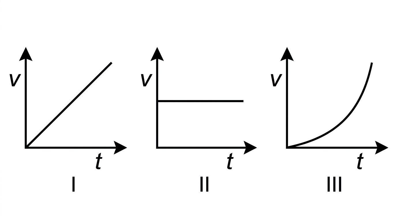
In which of these cases is the rate of change of the particle’s displacement constant?
A spacecraft accelerates at a rate of \(20.0 \, \text{m/s}^2\).
You are standing on a bathroom scale in an elevator. The elevator starts from rest on the first floor and accelerates up to the third floor, \(12 \, \text{m}\) above, in a time of \(6 \, \text{s}\). The scale reads \(800 \, \text{N}\). What is the mass of the person?
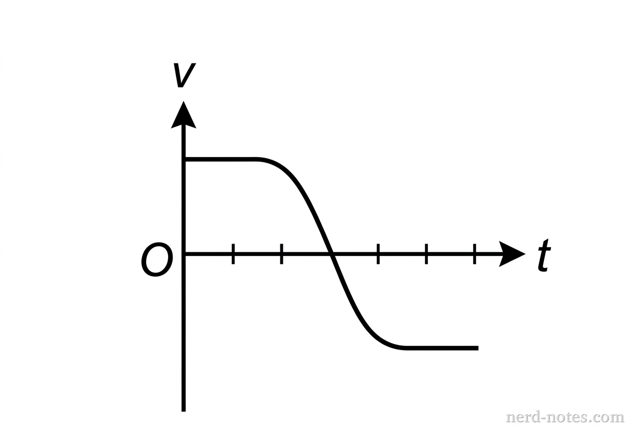
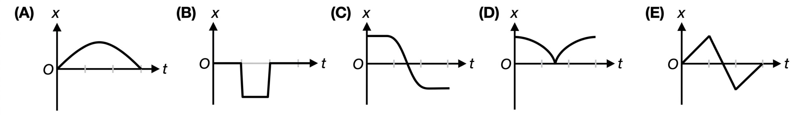
The graph above shows velocity \( v \) versus time \( t \) for an object in linear motion. Which of the following is a possible graph of position (\( x \)) versus time (\( t \)) for this object?
\(\text{Yes}\)
\(t = 9\,\text{s},\; \Delta x = 54\,\text{m}\)
\(\text{Runner B, }2.56\,\text{s}\)
By continuing you (1) agree to our Terms of Use and Terms of Sale and (2) consent to sharing your IP and browser information used by this site’s security protocols as outlined in our Privacy Policy.
| Kinematics | Forces |
|---|---|
| \(\Delta x = v_i t + \frac{1}{2} at^2\) | \(F = ma\) |
| \(v = v_i + at\) | \(F_g = \frac{G m_1 m_2}{r^2}\) |
| \(v^2 = v_i^2 + 2a \Delta x\) | \(f = \mu N\) |
| \(\Delta x = \frac{v_i + v}{2} t\) | \(F_s =-kx\) |
| \(v^2 = v_f^2 \,-\, 2a \Delta x\) |
| Circular Motion | Energy |
|---|---|
| \(F_c = \frac{mv^2}{r}\) | \(KE = \frac{1}{2} mv^2\) |
| \(a_c = \frac{v^2}{r}\) | \(PE = mgh\) |
| \(T = 2\pi \sqrt{\frac{r}{g}}\) | \(KE_i + PE_i = KE_f + PE_f\) |
| \(W = Fd \cos\theta\) |
| Momentum | Torque and Rotations |
|---|---|
| \(p = mv\) | \(\tau = r \cdot F \cdot \sin(\theta)\) |
| \(J = \Delta p\) | \(I = \sum mr^2\) |
| \(p_i = p_f\) | \(L = I \cdot \omega\) |
| Simple Harmonic Motion | Fluids |
|---|---|
| \(F = -kx\) | \(P = \frac{F}{A}\) |
| \(T = 2\pi \sqrt{\frac{l}{g}}\) | \(P_{\text{total}} = P_{\text{atm}} + \rho gh\) |
| \(T = 2\pi \sqrt{\frac{m}{k}}\) | \(Q = Av\) |
| \(x(t) = A \cos(\omega t + \phi)\) | \(F_b = \rho V g\) |
| \(a = -\omega^2 x\) | \(A_1v_1 = A_2v_2\) |
| Constant | Description |
|---|---|
| [katex]g[/katex] | Acceleration due to gravity, typically [katex]9.8 , \text{m/s}^2[/katex] on Earth’s surface |
| [katex]G[/katex] | Universal Gravitational Constant, [katex]6.674 \times 10^{-11} , \text{N} \cdot \text{m}^2/\text{kg}^2[/katex] |
| [katex]\mu_k[/katex] and [katex]\mu_s[/katex] | Coefficients of kinetic ([katex]\mu_k[/katex]) and static ([katex]\mu_s[/katex]) friction, dimensionless. Static friction ([katex]\mu_s[/katex]) is usually greater than kinetic friction ([katex]\mu_k[/katex]) as it resists the start of motion. |
| [katex]k[/katex] | Spring constant, in [katex]\text{N/m}[/katex] |
| [katex] M_E = 5.972 \times 10^{24} , \text{kg} [/katex] | Mass of the Earth |
| [katex] M_M = 7.348 \times 10^{22} , \text{kg} [/katex] | Mass of the Moon |
| [katex] M_M = 1.989 \times 10^{30} , \text{kg} [/katex] | Mass of the Sun |
| Variable | SI Unit |
|---|---|
| [katex]s[/katex] (Displacement) | [katex]\text{meters (m)}[/katex] |
| [katex]v[/katex] (Velocity) | [katex]\text{meters per second (m/s)}[/katex] |
| [katex]a[/katex] (Acceleration) | [katex]\text{meters per second squared (m/s}^2\text{)}[/katex] |
| [katex]t[/katex] (Time) | [katex]\text{seconds (s)}[/katex] |
| [katex]m[/katex] (Mass) | [katex]\text{kilograms (kg)}[/katex] |
| Variable | Derived SI Unit |
|---|---|
| [katex]F[/katex] (Force) | [katex]\text{newtons (N)}[/katex] |
| [katex]E[/katex], [katex]PE[/katex], [katex]KE[/katex] (Energy, Potential Energy, Kinetic Energy) | [katex]\text{joules (J)}[/katex] |
| [katex]P[/katex] (Power) | [katex]\text{watts (W)}[/katex] |
| [katex]p[/katex] (Momentum) | [katex]\text{kilogram meters per second (kgm/s)}[/katex] |
| [katex]\omega[/katex] (Angular Velocity) | [katex]\text{radians per second (rad/s)}[/katex] |
| [katex]\tau[/katex] (Torque) | [katex]\text{newton meters (Nm)}[/katex] |
| [katex]I[/katex] (Moment of Inertia) | [katex]\text{kilogram meter squared (kgm}^2\text{)}[/katex] |
| [katex]f[/katex] (Frequency) | [katex]\text{hertz (Hz)}[/katex] |
Metric Prefixes
Example of using unit analysis: Convert 5 kilometers to millimeters.
Start with the given measurement: [katex]\text{5 km}[/katex]
Use the conversion factors for kilometers to meters and meters to millimeters: [katex]\text{5 km} \times \frac{10^3 \, \text{m}}{1 \, \text{km}} \times \frac{10^3 \, \text{mm}}{1 \, \text{m}}[/katex]
Perform the multiplication: [katex]\text{5 km} \times \frac{10^3 \, \text{m}}{1 \, \text{km}} \times \frac{10^3 \, \text{mm}}{1 \, \text{m}} = 5 \times 10^3 \times 10^3 \, \text{mm}[/katex]
Simplify to get the final answer: [katex]\boxed{5 \times 10^6 \, \text{mm}}[/katex]
Prefix | Symbol | Power of Ten | Equivalent |
|---|---|---|---|
Pico- | p | [katex]10^{-12}[/katex] | 0.000000000001 |
Nano- | n | [katex]10^{-9}[/katex] | 0.000000001 |
Micro- | µ | [katex]10^{-6}[/katex] | 0.000001 |
Milli- | m | [katex]10^{-3}[/katex] | 0.001 |
Centi- | c | [katex]10^{-2}[/katex] | 0.01 |
Deci- | d | [katex]10^{-1}[/katex] | 0.1 |
(Base unit) | – | [katex]10^{0}[/katex] | 1 |
Deca- or Deka- | da | [katex]10^{1}[/katex] | 10 |
Hecto- | h | [katex]10^{2}[/katex] | 100 |
Kilo- | k | [katex]10^{3}[/katex] | 1,000 |
Mega- | M | [katex]10^{6}[/katex] | 1,000,000 |
Giga- | G | [katex]10^{9}[/katex] | 1,000,000,000 |
Tera- | T | [katex]10^{12}[/katex] | 1,000,000,000,000 |
One price to unlock most advanced version of Phy across all our tools.
per month
Billed Monthly. Cancel Anytime.
Try our free calculator to see what you need to get a 5 on the 2026 AP Physics 1 exam.
A quick explanation
Credits are used to grade your FRQs and GQs. Pro users get unlimited credits.
Submitting counts as 1 attempt.
Viewing answers or explanations count as a failed attempts.
Phy gives partial credit if needed
MCQs and GQs are are 1 point each. FRQs will state points for each part.
Phy customizes problem explanations based on what you struggle with. Just hit the explanation button to see.
Understand you mistakes quicker.

Phy automatically provides feedback so you can improve your responses.
10 Free Credits To Get You Started

By continuing you agree to nerd-notes.com Terms of Service, Privacy Policy, and our usage of user data.
Feeling uneasy about your next physics test? We'll boost your grade in 3 lessons or less—guaranteed

NEW! PHY AI accurately solves all questions
🔥 Get up to 30% off Elite Physics Tutoring
🧠 NEW! Learn Physics From Scratch Self Paced Course
🎯 Need exam style practice questions?
