| Step | Formula Derivation | Reasoning |
|---|---|---|
| 1 | [katex] a_{\text{centripetal}} = \frac{v^2}{r} [/katex] | Centripetal acceleration formula, where [katex] v [/katex] is velocity and [katex] r [/katex] is the radius. |
| 2 | [katex] v = \frac{2\pi r}{T} [/katex] | Velocity formula for uniform circular motion, with [katex] T [/katex] as the period. |
| 3 | [katex] a_{\text{centripetal}} = \frac{\left(\frac{2\pi r}{T}\right)^2}{r} = \frac{4\pi^2 r}{T^2} [/katex] | Substituting the expression for [katex] v [/katex] from Step 2 into the centripetal acceleration formula. |
| 4 | [katex] a_{\text{centripetal, new}} = \frac{4\pi^2 (R/3)}{T^2} = \frac{4\pi^2 R}{3T^2} [/katex] | Applying the formula to the new radius [katex] R/3 [/katex]. |
| 5 | [katex] \text{Ratio} = \frac{a_{\text{centripetal, new}}}{a_{\text{centripetal, original}}} = \frac{\frac{4\pi^2 R}{3T^2}}{\frac{4\pi^2 R}{T^2}} = \frac{1}{3} [/katex] | Calculating the ratio of new acceleration to original acceleration. |
| 6 | [katex] \boxed{\text{The centripetal acceleration decreases by a factor of 3.}} [/katex] | Conclusion based on the ratio calculated in Step 5. |
A Major Upgrade To Phy Is Coming Soon — Stay Tuned
We'll help clarify entire units in one hour or less — guaranteed.
A 2.0 kg ball on the end of a 0.65 m long string is moving in a vertical circle. At the bottom of the circle, its speed is 4.0 m/s. Find the tension in the string.
A communications satellite orbits the Earth at an altitude of \(35{,}000 \, \text{km}\) above the Earth’s surface. Take the mass of Earth to be \(6 \times 10^{24} \, \text{kg}\) and the radius of Earth to be \(6.4 \times 10^6 \, \text{m}\). What is the satellite’s velocity?
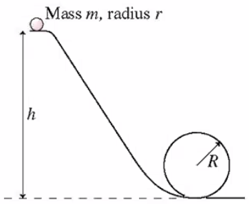
In the figure above, the marble rolls down the track and around a loop-the-loop of radius \( R \). The marble has mass \( m \) and radius \( r \). What minimum height \( h_{min} \) must the track have for the marble to make it around the loop-the-loop without falling off? Express your answer in terms of the variables \( R \) and \( r \).
Young David experimented with slings before tackling Goliath. He found that he could develop an angular speed of \( 8.0 \) \( \text{rev/s} \) in a sling \( 0.60 \) \( \text{m} \) long. If he increased the length to \( 0.90 \) \( \text{m} \), he could revolve the sling only \( 6.0 \) times per second.
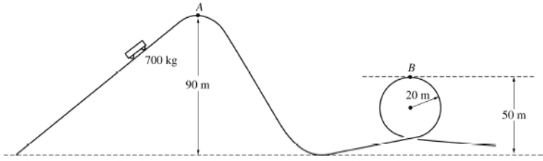
A roller coaster ride at an amusement park lifts a car of mass \( 700 \, \text{kg} \) to point \( A \) at a height of \( 90 \, \text{m} \) above the lowest point on the track, as shown above. The car starts from rest at \( A \), rolls with negligible friction down the incline and follows the track around a loop of radius \( 20 \, \text{m} \). Point \( B \), the highest point on the loop, is at a height of \( 50 \, \text{m} \) above the lowest point on the track.
A car is going over the top of a hill whose curvature approximates a circle of radius \( 350 \) \( \text{m} \). At what velocity will the occupants of the car appear to weigh \( 10\% \) less than their normal weight?
Why do pilots sometimes black out while pulling out at the bottom of a dive?
A \(1.00 \, \text{kg}\) mass is attached to a \(0.800 \, \text{m}\) long string and spun in a vertical circle. The mass completes \(2.00\) revolutions in \(1.00 \, \text{s}\).
A concrete highway curve of radius \(60.0 \, \text{m}\) is banked at a \(12.0^\circ\) angle. What is the maximum speed with which a \(1300 \, \text{kg}\) rubber-tired car can take this curve without sliding? (Take the static coefficient of friction of rubber on concrete to be \(1.0\).)
A car is going through a dip in the road whose curvature approximates a circle of radius \( 200 \) \( \text{m} \). At what velocity will the occupants of the car appear to weigh \( 20\% \) more than their normal weight \( (1.2\,W) \)?
By continuing you (1) agree to our Terms of Use and Terms of Sale and (2) consent to sharing your IP and browser information used by this site’s security protocols as outlined in our Privacy Policy.
| Kinematics | Forces |
|---|---|
| \(\Delta x = v_i t + \frac{1}{2} at^2\) | \(F = ma\) |
| \(v = v_i + at\) | \(F_g = \frac{G m_1 m_2}{r^2}\) |
| \(v^2 = v_i^2 + 2a \Delta x\) | \(f = \mu N\) |
| \(\Delta x = \frac{v_i + v}{2} t\) | \(F_s =-kx\) |
| \(v^2 = v_f^2 \,-\, 2a \Delta x\) |
| Circular Motion | Energy |
|---|---|
| \(F_c = \frac{mv^2}{r}\) | \(KE = \frac{1}{2} mv^2\) |
| \(a_c = \frac{v^2}{r}\) | \(PE = mgh\) |
| \(T = 2\pi \sqrt{\frac{r}{g}}\) | \(KE_i + PE_i = KE_f + PE_f\) |
| \(W = Fd \cos\theta\) |
| Momentum | Torque and Rotations |
|---|---|
| \(p = mv\) | \(\tau = r \cdot F \cdot \sin(\theta)\) |
| \(J = \Delta p\) | \(I = \sum mr^2\) |
| \(p_i = p_f\) | \(L = I \cdot \omega\) |
| Simple Harmonic Motion | Fluids |
|---|---|
| \(F = -kx\) | \(P = \frac{F}{A}\) |
| \(T = 2\pi \sqrt{\frac{l}{g}}\) | \(P_{\text{total}} = P_{\text{atm}} + \rho gh\) |
| \(T = 2\pi \sqrt{\frac{m}{k}}\) | \(Q = Av\) |
| \(x(t) = A \cos(\omega t + \phi)\) | \(F_b = \rho V g\) |
| \(a = -\omega^2 x\) | \(A_1v_1 = A_2v_2\) |
| Constant | Description |
|---|---|
| [katex]g[/katex] | Acceleration due to gravity, typically [katex]9.8 , \text{m/s}^2[/katex] on Earth’s surface |
| [katex]G[/katex] | Universal Gravitational Constant, [katex]6.674 \times 10^{-11} , \text{N} \cdot \text{m}^2/\text{kg}^2[/katex] |
| [katex]\mu_k[/katex] and [katex]\mu_s[/katex] | Coefficients of kinetic ([katex]\mu_k[/katex]) and static ([katex]\mu_s[/katex]) friction, dimensionless. Static friction ([katex]\mu_s[/katex]) is usually greater than kinetic friction ([katex]\mu_k[/katex]) as it resists the start of motion. |
| [katex]k[/katex] | Spring constant, in [katex]\text{N/m}[/katex] |
| [katex] M_E = 5.972 \times 10^{24} , \text{kg} [/katex] | Mass of the Earth |
| [katex] M_M = 7.348 \times 10^{22} , \text{kg} [/katex] | Mass of the Moon |
| [katex] M_M = 1.989 \times 10^{30} , \text{kg} [/katex] | Mass of the Sun |
| Variable | SI Unit |
|---|---|
| [katex]s[/katex] (Displacement) | [katex]\text{meters (m)}[/katex] |
| [katex]v[/katex] (Velocity) | [katex]\text{meters per second (m/s)}[/katex] |
| [katex]a[/katex] (Acceleration) | [katex]\text{meters per second squared (m/s}^2\text{)}[/katex] |
| [katex]t[/katex] (Time) | [katex]\text{seconds (s)}[/katex] |
| [katex]m[/katex] (Mass) | [katex]\text{kilograms (kg)}[/katex] |
| Variable | Derived SI Unit |
|---|---|
| [katex]F[/katex] (Force) | [katex]\text{newtons (N)}[/katex] |
| [katex]E[/katex], [katex]PE[/katex], [katex]KE[/katex] (Energy, Potential Energy, Kinetic Energy) | [katex]\text{joules (J)}[/katex] |
| [katex]P[/katex] (Power) | [katex]\text{watts (W)}[/katex] |
| [katex]p[/katex] (Momentum) | [katex]\text{kilogram meters per second (kgm/s)}[/katex] |
| [katex]\omega[/katex] (Angular Velocity) | [katex]\text{radians per second (rad/s)}[/katex] |
| [katex]\tau[/katex] (Torque) | [katex]\text{newton meters (Nm)}[/katex] |
| [katex]I[/katex] (Moment of Inertia) | [katex]\text{kilogram meter squared (kgm}^2\text{)}[/katex] |
| [katex]f[/katex] (Frequency) | [katex]\text{hertz (Hz)}[/katex] |
Metric Prefixes
Example of using unit analysis: Convert 5 kilometers to millimeters.
Start with the given measurement: [katex]\text{5 km}[/katex]
Use the conversion factors for kilometers to meters and meters to millimeters: [katex]\text{5 km} \times \frac{10^3 \, \text{m}}{1 \, \text{km}} \times \frac{10^3 \, \text{mm}}{1 \, \text{m}}[/katex]
Perform the multiplication: [katex]\text{5 km} \times \frac{10^3 \, \text{m}}{1 \, \text{km}} \times \frac{10^3 \, \text{mm}}{1 \, \text{m}} = 5 \times 10^3 \times 10^3 \, \text{mm}[/katex]
Simplify to get the final answer: [katex]\boxed{5 \times 10^6 \, \text{mm}}[/katex]
Prefix | Symbol | Power of Ten | Equivalent |
|---|---|---|---|
Pico- | p | [katex]10^{-12}[/katex] | 0.000000000001 |
Nano- | n | [katex]10^{-9}[/katex] | 0.000000001 |
Micro- | µ | [katex]10^{-6}[/katex] | 0.000001 |
Milli- | m | [katex]10^{-3}[/katex] | 0.001 |
Centi- | c | [katex]10^{-2}[/katex] | 0.01 |
Deci- | d | [katex]10^{-1}[/katex] | 0.1 |
(Base unit) | – | [katex]10^{0}[/katex] | 1 |
Deca- or Deka- | da | [katex]10^{1}[/katex] | 10 |
Hecto- | h | [katex]10^{2}[/katex] | 100 |
Kilo- | k | [katex]10^{3}[/katex] | 1,000 |
Mega- | M | [katex]10^{6}[/katex] | 1,000,000 |
Giga- | G | [katex]10^{9}[/katex] | 1,000,000,000 |
Tera- | T | [katex]10^{12}[/katex] | 1,000,000,000,000 |
One price to unlock most advanced version of Phy across all our tools.
per month
Billed Monthly. Cancel Anytime.
We crafted THE Ultimate A.P Physics 1 Program so you can learn faster and score higher.
Try our free calculator to see what you need to get a 5 on the 2026 AP Physics 1 exam.
A quick explanation
Credits are used to grade your FRQs and GQs. Pro users get unlimited credits.
Submitting counts as 1 attempt.
Viewing answers or explanations count as a failed attempts.
Phy gives partial credit if needed
MCQs and GQs are are 1 point each. FRQs will state points for each part.
Phy customizes problem explanations based on what you struggle with. Just hit the explanation button to see.
Understand you mistakes quicker.

Phy automatically provides feedback so you can improve your responses.
10 Free Credits To Get You Started

By continuing you agree to nerd-notes.com Terms of Service, Privacy Policy, and our usage of user data.
Feeling uneasy about your next physics test? We'll boost your grade in 3 lessons or less—guaranteed

NEW! PHY AI accurately solves all questions
🔥 Get up to 30% off Elite Physics Tutoring
🧠 NEW! Learn Physics From Scratch Self Paced Course
🎯 Need exam style practice questions?
