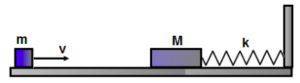
A small block moving with a constant speed \(v\) collides inelastically with a block \(M\) attached to one end of a spring \(k\). The other end of the spring is connected to a stationary wall. Ignore friction between the blocks and the surface.
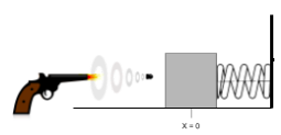
A bullet (mass: \(0.05 \, \text{kg}\)) is fired horizontally (\(v = 200 \, \text{m/s}\)) at a block (mass: \(1.3 \, \text{kg}\)) initially at rest on a frictionless surface. The block is attached to a spring (\(k = 2500 \, \text{N/m}\)). The bullet becomes embedded. Calculate:

A simple pendulum oscillates with amplitude \(A\) and period \(T\), as represented on the graph above. Which option best represents the magnitude of the pendulum’s velocity \(v\) and acceleration \(a\) at time \(\frac{T}{2}\)?


