| Step | Derivation/Formula | Reasoning |
|---|---|---|
| 1 | \[F_f = \mu mg\] | The maximum braking force is the kinetic friction between wheels and surface, with coefficient \(\mu\). |
| 2 | \[ma = F_f\] | Apply Newton\’s second law; the net braking force produces a deceleration \(a\). |
| 3 | \[a = \mu g\] | Solving the previous step for \(a\) shows it depends only on \(\mu\) and \(g\); mass cancels. |
| 4 | \[v_x^2 = v_i^2 + 2a\Delta x\] | Use the constant‑acceleration kinematic relation connecting velocities, acceleration, and displacement. |
| 5 | \[0 = v_i^2 – 2\mu g d\] | Set final speed \(v_x = 0\) for a full stop, replace \(a\) with \(-\mu g\), and let stopping distance be \(d\). |
| 6 | \[d = \dfrac{v_i^2}{2\mu g}\] | Algebraically solve for the stopping distance. |
| 7 | \[\boxed{d \propto \dfrac{1}{\mu}}\] | The derived expression shows stopping distance is inversely proportional to the friction coefficient; vehicle mass is irrelevant, when it comes to stopping distance. |
| 8 | \[\mu_{\text{truck}} \approx 0.7,\quad \mu_{\text{train}} \approx 0.2\] | Typical values: rubber tires on asphalt have a much higher \(\mu\) than steel wheels on steel rails. |
| 9 | \[d_{\text{truck}} = \dfrac{v_i^2}{2\cdot0.7 g} < d_{\text{train}} = \dfrac{v_i^2}{2\cdot0.2 g}\] | A larger \(\mu\) for the truck yields a substantially shorter stopping distance than for the train at the same speed \(v_i\). |
A Major Upgrade To Phy Is Coming Soon — Stay Tuned

We'll help clarify entire units in one hour or less — guaranteed.
A self paced course with videos, problems sets, and everything you need to get a 5. Trusted by over 15k students and over 200 schools.
A child on Earth has a weight of \(500 \, \text{N}\). Determine the weight of the child if the Earth were to triple in both mass and radius (\(3M\) and \(3r\)).
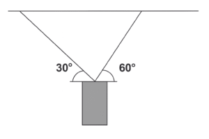
Two wires support an unknown mass as shown in the diagram. The tension in the left wire is measured to be \( 17.5 \) \( \text{N} \) and the tension in the right wire is \( 30.3 \) \( \text{N} \). The left wire makes an angle of \( 30^{\circ} \) with the horizontal, and the right wire makes an angle of \( 60^{\circ} \) with the horizontal. What is the mass of the object?
A box rests on the (frictionless) bed of a truck. The truck driver starts the truck and accelerates forward. The box immediately starts to slide toward the rear of the truck bed.
Which of the following statements about the acceleration due to gravity is TRUE?
A car is driving to the right at \( 20 \) \( \text{m/s} \). A motorcycle starts \( 30 \) \( \text{m} \) behind the car and is moving at \( 30 \) \( \text{m/s} \) in the same direction.
Two balls have their centers \( 2.0 \) \( \text{m} \) apart. One ball has a mass of \( 8.0 \) \( \text{kg} \). The other has a mass of \( 6.0 \) \( \text{kg} \). What is the gravitational force between them?
A “doomsday” asteroid with a mass of \( 1010 \, \text{kg} \) is hurtling through space. Unless the asteroid’s speed is changed by about \( 0.20 \, \text{cm/s} \), it will collide with Earth and cause tremendous damage. Researchers suggest that a small “space tug” sent to the asteroid’s surface could exert a gentle constant force of \( 2.5 \, \text{N} \). For how long must this force act?
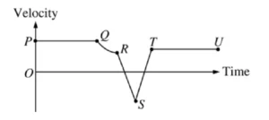 The graph above shows velocity as a function of time for an object moving along a straight line. For which of the following sections of the graph is the acceleration constant and nonzero?
When the speed of a rear-wheel-drive car is increasing on a horizontal road, what is the direction of the frictional force on the tires?
A red car, initially at rest, travels east with an acceleration of \( 3.5 \, \text{m/s}^2 \). At the same time as the red car starts to move, a blue car is traveling west at \( 15 \, \text{m/s} \) and accelerating at \( 1.2 \, \text{m/s}^2 \). If they are \( 600 \, \text{m} \) apart the moment the red car starts to move and they are traveling towards each other, where and when will they meet?
It must be that \(\mu_{\text{truck}} > \mu_{\text{train}}\).
By continuing you (1) agree to our Terms of Use and Terms of Sale and (2) consent to sharing your IP and browser information used by this site’s security protocols as outlined in our Privacy Policy.
| Kinematics | Forces |
|---|---|
| \(\Delta x = v_i t + \frac{1}{2} at^2\) | \(F = ma\) |
| \(v = v_i + at\) | \(F_g = \frac{G m_1 m_2}{r^2}\) |
| \(v^2 = v_i^2 + 2a \Delta x\) | \(f = \mu N\) |
| \(\Delta x = \frac{v_i + v}{2} t\) | \(F_s =-kx\) |
| \(v^2 = v_f^2 \,-\, 2a \Delta x\) |
| Circular Motion | Energy |
|---|---|
| \(F_c = \frac{mv^2}{r}\) | \(KE = \frac{1}{2} mv^2\) |
| \(a_c = \frac{v^2}{r}\) | \(PE = mgh\) |
| \(T = 2\pi \sqrt{\frac{r}{g}}\) | \(KE_i + PE_i = KE_f + PE_f\) |
| \(W = Fd \cos\theta\) |
| Momentum | Torque and Rotations |
|---|---|
| \(p = mv\) | \(\tau = r \cdot F \cdot \sin(\theta)\) |
| \(J = \Delta p\) | \(I = \sum mr^2\) |
| \(p_i = p_f\) | \(L = I \cdot \omega\) |
| Simple Harmonic Motion | Fluids |
|---|---|
| \(F = -kx\) | \(P = \frac{F}{A}\) |
| \(T = 2\pi \sqrt{\frac{l}{g}}\) | \(P_{\text{total}} = P_{\text{atm}} + \rho gh\) |
| \(T = 2\pi \sqrt{\frac{m}{k}}\) | \(Q = Av\) |
| \(x(t) = A \cos(\omega t + \phi)\) | \(F_b = \rho V g\) |
| \(a = -\omega^2 x\) | \(A_1v_1 = A_2v_2\) |
| Constant | Description |
|---|---|
| [katex]g[/katex] | Acceleration due to gravity, typically [katex]9.8 , \text{m/s}^2[/katex] on Earth’s surface |
| [katex]G[/katex] | Universal Gravitational Constant, [katex]6.674 \times 10^{-11} , \text{N} \cdot \text{m}^2/\text{kg}^2[/katex] |
| [katex]\mu_k[/katex] and [katex]\mu_s[/katex] | Coefficients of kinetic ([katex]\mu_k[/katex]) and static ([katex]\mu_s[/katex]) friction, dimensionless. Static friction ([katex]\mu_s[/katex]) is usually greater than kinetic friction ([katex]\mu_k[/katex]) as it resists the start of motion. |
| [katex]k[/katex] | Spring constant, in [katex]\text{N/m}[/katex] |
| [katex] M_E = 5.972 \times 10^{24} , \text{kg} [/katex] | Mass of the Earth |
| [katex] M_M = 7.348 \times 10^{22} , \text{kg} [/katex] | Mass of the Moon |
| [katex] M_M = 1.989 \times 10^{30} , \text{kg} [/katex] | Mass of the Sun |
| Variable | SI Unit |
|---|---|
| [katex]s[/katex] (Displacement) | [katex]\text{meters (m)}[/katex] |
| [katex]v[/katex] (Velocity) | [katex]\text{meters per second (m/s)}[/katex] |
| [katex]a[/katex] (Acceleration) | [katex]\text{meters per second squared (m/s}^2\text{)}[/katex] |
| [katex]t[/katex] (Time) | [katex]\text{seconds (s)}[/katex] |
| [katex]m[/katex] (Mass) | [katex]\text{kilograms (kg)}[/katex] |
| Variable | Derived SI Unit |
|---|---|
| [katex]F[/katex] (Force) | [katex]\text{newtons (N)}[/katex] |
| [katex]E[/katex], [katex]PE[/katex], [katex]KE[/katex] (Energy, Potential Energy, Kinetic Energy) | [katex]\text{joules (J)}[/katex] |
| [katex]P[/katex] (Power) | [katex]\text{watts (W)}[/katex] |
| [katex]p[/katex] (Momentum) | [katex]\text{kilogram meters per second (kgm/s)}[/katex] |
| [katex]\omega[/katex] (Angular Velocity) | [katex]\text{radians per second (rad/s)}[/katex] |
| [katex]\tau[/katex] (Torque) | [katex]\text{newton meters (Nm)}[/katex] |
| [katex]I[/katex] (Moment of Inertia) | [katex]\text{kilogram meter squared (kgm}^2\text{)}[/katex] |
| [katex]f[/katex] (Frequency) | [katex]\text{hertz (Hz)}[/katex] |
Metric Prefixes
Example of using unit analysis: Convert 5 kilometers to millimeters.
Start with the given measurement: [katex]\text{5 km}[/katex]
Use the conversion factors for kilometers to meters and meters to millimeters: [katex]\text{5 km} \times \frac{10^3 \, \text{m}}{1 \, \text{km}} \times \frac{10^3 \, \text{mm}}{1 \, \text{m}}[/katex]
Perform the multiplication: [katex]\text{5 km} \times \frac{10^3 \, \text{m}}{1 \, \text{km}} \times \frac{10^3 \, \text{mm}}{1 \, \text{m}} = 5 \times 10^3 \times 10^3 \, \text{mm}[/katex]
Simplify to get the final answer: [katex]\boxed{5 \times 10^6 \, \text{mm}}[/katex]
Prefix | Symbol | Power of Ten | Equivalent |
|---|---|---|---|
Pico- | p | [katex]10^{-12}[/katex] | 0.000000000001 |
Nano- | n | [katex]10^{-9}[/katex] | 0.000000001 |
Micro- | µ | [katex]10^{-6}[/katex] | 0.000001 |
Milli- | m | [katex]10^{-3}[/katex] | 0.001 |
Centi- | c | [katex]10^{-2}[/katex] | 0.01 |
Deci- | d | [katex]10^{-1}[/katex] | 0.1 |
(Base unit) | – | [katex]10^{0}[/katex] | 1 |
Deca- or Deka- | da | [katex]10^{1}[/katex] | 10 |
Hecto- | h | [katex]10^{2}[/katex] | 100 |
Kilo- | k | [katex]10^{3}[/katex] | 1,000 |
Mega- | M | [katex]10^{6}[/katex] | 1,000,000 |
Giga- | G | [katex]10^{9}[/katex] | 1,000,000,000 |
Tera- | T | [katex]10^{12}[/katex] | 1,000,000,000,000 |
One price to unlock most advanced version of Phy across all our tools.
per month
Billed Monthly. Cancel Anytime.
Try our free calculator to see what you need to get a 5 on the 2026 AP Physics 1 exam.
A quick explanation
Credits are used to grade your FRQs and GQs. Pro users get unlimited credits.
Submitting counts as 1 attempt.
Viewing answers or explanations count as a failed attempts.
Phy gives partial credit if needed
MCQs and GQs are are 1 point each. FRQs will state points for each part.
Phy customizes problem explanations based on what you struggle with. Just hit the explanation button to see.
Understand you mistakes quicker.

Phy automatically provides feedback so you can improve your responses.
10 Free Credits To Get You Started

By continuing you agree to nerd-notes.com Terms of Service, Privacy Policy, and our usage of user data.
Feeling uneasy about your next physics test? We'll boost your grade in 3 lessons or less—guaranteed

NEW! PHY AI accurately solves all questions
🔥 Get up to 30% off Elite Physics Tutoring
🧠 NEW! Learn Physics From Scratch Self Paced Course
🎯 Need exam style practice questions?
