0 attempts
0% avg
| Step | Derivation/Formula | Reasoning |
|---|---|---|
| 1 | \[\Delta L_A = 10\,\text{kg}\cdot\text{m}^2/\text{s}\] | The graph shows disk A rises from \(0\) to \(10\,\text{kg}\cdot\text{m}^2/\text{s}\) between \(t = 0\,\text{s}\) and \(t = 5\,\text{s}\), so \(\Delta L_A = 10\). |
| 2 | \[\Delta L_B = 20\,\text{kg}\cdot\text{m}^2/\text{s}\] | The graph shows disk B rises from \(0\) to \(20\,\text{kg}\cdot\text{m}^2/\text{s}\) in the same time interval, so \(\Delta L_B = 20\). |
| 3 | \[\tau_{\text{avg}} = \frac{\Delta L}{\Delta t}\] | Average net torque equals the change in angular momentum divided by the time interval (algebraic definition, no calculus needed). |
| 4 | \[\tau_A = \frac{10}{5} = 2\,\text{N}\cdot\text{m}\] | Substituting \(\Delta L_A = 10\) and \(\Delta t = 5\,\text{s}\) gives the average torque on disk A. |
| 5 | \[\tau_B = \frac{20}{5} = 4\,\text{N}\cdot\text{m}\] | Substituting \(\Delta L_B = 20\) and \(\Delta t = 5\,\text{s}\) gives the average torque on disk B. |
| 6 | \[\tau_B = 2\tau_A\] | Using \(\tau_A = 2\) and \(\tau_B = 4\) shows the required relationship. The disks’ different rotational inertias are irrelevant because inertia cancels in \(\Delta L\). |
| Incorrect Option (a) | \[\tau_B = 4\tau_A\] | This predicts \(\tau_B = 8\,\text{N}\cdot\text{m}\), which contradicts the calculated \(\tau_B = 4\,\text{N}\cdot\text{m}\). |
| Incorrect Option (c) | \[\tau_B = \tfrac{1}{2}\tau_A\] | This would give \(\tau_B = 1\,\text{N}\cdot\text{m}\), far below the value obtained from the graph. |
| Incorrect Option (d) | \[\tau_B = \tfrac{1}{4}\tau_A\] | This would give \(\tau_B = 0.5\,\text{N}\cdot\text{m}\), also inconsistent with the calculated \(4\,\text{N}\cdot\text{m}\). |
Just ask: "Help me solve this problem."
We'll help clarify entire units in one hour or less — guaranteed.
How long does it take for a rotating object to speed up from 15.0 rad/s to 33.3 rad/s if it has a uniform angular acceleration of 3.45 rad/s2?
A horizontal, uniform board of weight 125 N and length 4 m is supported by vertical chains at each end. A person weighing 500 N is sitting on the board. The tension in the right chain is 250 N. How far from the left end of the board is the person sitting?
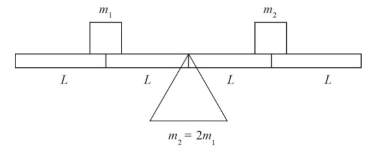
The system above is NOT balanced since \(m_2\) is twice the mass of \(m_1\). Which of the following changes would NOT balance the system so that there is 0 net torque? Assume the plank has no mass of its own.
To increase the moment of inertia of a body about an axis, you must
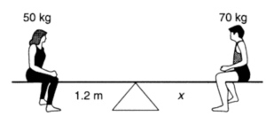
A \( 50 \, \text{kg} \) person is sitting on a seesaw \( 1.2 \, \text{m} \) from the balance point. On the other side, a \( 70 \, \text{kg} \) person is balanced. How far from the balance point is the second person sitting?
Two workers are holding a thin plate with length \(5 \, \text{m}\) and height \(2 \, \text{m}\) at rest by supporting the plate in the bottom corners. The workers are standing at rest on a slope of \(10^\circ\). Treat these supporting forces as vertical normal forces and calculate their magnitudes and state if both workers are sharing “the job” fairly.
A car is moving up the side of a circular roller coaster loop of radius \( 12 \) \( \text{m} \). The angular velocity is \( 1.8 \) \( \text{rad/s} \) and angular acceleration is \( -0.82 \) \( \text{rad/s}^2 \). The car is at the same elevation as the center of the loop. Find the magnitude and direction (relative to the horizontal) of the acceleration.
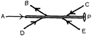
Five forces act on a rod that is free to pivot at point \( P \), as shown in the figure. Which of these forces is producing a counter-clockwise torque about point \( P \)?
When the speed of a rear-drive car is increasing on a horizontal road, what is the direction of the frictional force on the tires?
By continuing you (1) agree to our Terms of Use and Terms of Sale and (2) consent to sharing your IP and browser information used by this site’s security protocols as outlined in our Privacy Policy.
| Kinematics | Forces |
|---|---|
| \(\Delta x = v_i t + \frac{1}{2} at^2\) | \(F = ma\) |
| \(v = v_i + at\) | \(F_g = \frac{G m_1 m_2}{r^2}\) |
| \(v^2 = v_i^2 + 2a \Delta x\) | \(f = \mu N\) |
| \(\Delta x = \frac{v_i + v}{2} t\) | \(F_s =-kx\) |
| \(v^2 = v_f^2 \,-\, 2a \Delta x\) |
| Circular Motion | Energy |
|---|---|
| \(F_c = \frac{mv^2}{r}\) | \(KE = \frac{1}{2} mv^2\) |
| \(a_c = \frac{v^2}{r}\) | \(PE = mgh\) |
| \(T = 2\pi \sqrt{\frac{r}{g}}\) | \(KE_i + PE_i = KE_f + PE_f\) |
| \(W = Fd \cos\theta\) |
| Momentum | Torque and Rotations |
|---|---|
| \(p = mv\) | \(\tau = r \cdot F \cdot \sin(\theta)\) |
| \(J = \Delta p\) | \(I = \sum mr^2\) |
| \(p_i = p_f\) | \(L = I \cdot \omega\) |
| Simple Harmonic Motion | Fluids |
|---|---|
| \(F = -kx\) | \(P = \frac{F}{A}\) |
| \(T = 2\pi \sqrt{\frac{l}{g}}\) | \(P_{\text{total}} = P_{\text{atm}} + \rho gh\) |
| \(T = 2\pi \sqrt{\frac{m}{k}}\) | \(Q = Av\) |
| \(x(t) = A \cos(\omega t + \phi)\) | \(F_b = \rho V g\) |
| \(a = -\omega^2 x\) | \(A_1v_1 = A_2v_2\) |
| Constant | Description |
|---|---|
| [katex]g[/katex] | Acceleration due to gravity, typically [katex]9.8 , \text{m/s}^2[/katex] on Earth’s surface |
| [katex]G[/katex] | Universal Gravitational Constant, [katex]6.674 \times 10^{-11} , \text{N} \cdot \text{m}^2/\text{kg}^2[/katex] |
| [katex]\mu_k[/katex] and [katex]\mu_s[/katex] | Coefficients of kinetic ([katex]\mu_k[/katex]) and static ([katex]\mu_s[/katex]) friction, dimensionless. Static friction ([katex]\mu_s[/katex]) is usually greater than kinetic friction ([katex]\mu_k[/katex]) as it resists the start of motion. |
| [katex]k[/katex] | Spring constant, in [katex]\text{N/m}[/katex] |
| [katex] M_E = 5.972 \times 10^{24} , \text{kg} [/katex] | Mass of the Earth |
| [katex] M_M = 7.348 \times 10^{22} , \text{kg} [/katex] | Mass of the Moon |
| [katex] M_M = 1.989 \times 10^{30} , \text{kg} [/katex] | Mass of the Sun |
| Variable | SI Unit |
|---|---|
| [katex]s[/katex] (Displacement) | [katex]\text{meters (m)}[/katex] |
| [katex]v[/katex] (Velocity) | [katex]\text{meters per second (m/s)}[/katex] |
| [katex]a[/katex] (Acceleration) | [katex]\text{meters per second squared (m/s}^2\text{)}[/katex] |
| [katex]t[/katex] (Time) | [katex]\text{seconds (s)}[/katex] |
| [katex]m[/katex] (Mass) | [katex]\text{kilograms (kg)}[/katex] |
| Variable | Derived SI Unit |
|---|---|
| [katex]F[/katex] (Force) | [katex]\text{newtons (N)}[/katex] |
| [katex]E[/katex], [katex]PE[/katex], [katex]KE[/katex] (Energy, Potential Energy, Kinetic Energy) | [katex]\text{joules (J)}[/katex] |
| [katex]P[/katex] (Power) | [katex]\text{watts (W)}[/katex] |
| [katex]p[/katex] (Momentum) | [katex]\text{kilogram meters per second (kgm/s)}[/katex] |
| [katex]\omega[/katex] (Angular Velocity) | [katex]\text{radians per second (rad/s)}[/katex] |
| [katex]\tau[/katex] (Torque) | [katex]\text{newton meters (Nm)}[/katex] |
| [katex]I[/katex] (Moment of Inertia) | [katex]\text{kilogram meter squared (kgm}^2\text{)}[/katex] |
| [katex]f[/katex] (Frequency) | [katex]\text{hertz (Hz)}[/katex] |
Metric Prefixes
Example of using unit analysis: Convert 5 kilometers to millimeters.
Start with the given measurement: [katex]\text{5 km}[/katex]
Use the conversion factors for kilometers to meters and meters to millimeters: [katex]\text{5 km} \times \frac{10^3 \, \text{m}}{1 \, \text{km}} \times \frac{10^3 \, \text{mm}}{1 \, \text{m}}[/katex]
Perform the multiplication: [katex]\text{5 km} \times \frac{10^3 \, \text{m}}{1 \, \text{km}} \times \frac{10^3 \, \text{mm}}{1 \, \text{m}} = 5 \times 10^3 \times 10^3 \, \text{mm}[/katex]
Simplify to get the final answer: [katex]\boxed{5 \times 10^6 \, \text{mm}}[/katex]
Prefix | Symbol | Power of Ten | Equivalent |
|---|---|---|---|
Pico- | p | [katex]10^{-12}[/katex] | 0.000000000001 |
Nano- | n | [katex]10^{-9}[/katex] | 0.000000001 |
Micro- | µ | [katex]10^{-6}[/katex] | 0.000001 |
Milli- | m | [katex]10^{-3}[/katex] | 0.001 |
Centi- | c | [katex]10^{-2}[/katex] | 0.01 |
Deci- | d | [katex]10^{-1}[/katex] | 0.1 |
(Base unit) | – | [katex]10^{0}[/katex] | 1 |
Deca- or Deka- | da | [katex]10^{1}[/katex] | 10 |
Hecto- | h | [katex]10^{2}[/katex] | 100 |
Kilo- | k | [katex]10^{3}[/katex] | 1,000 |
Mega- | M | [katex]10^{6}[/katex] | 1,000,000 |
Giga- | G | [katex]10^{9}[/katex] | 1,000,000,000 |
Tera- | T | [katex]10^{12}[/katex] | 1,000,000,000,000 |
One price to unlock most advanced version of Phy across all our tools.
per month
Billed Monthly. Cancel Anytime.
We crafted THE Ultimate A.P Physics 1 Program so you can learn faster and score higher.
Try our free calculator to see what you need to get a 5 on the 2026 AP Physics 1 exam.
A quick explanation
Credits are used to grade your FRQs and GQs. Pro users get unlimited credits.
Submitting counts as 1 attempt.
Viewing answers or explanations count as a failed attempts.
Phy gives partial credit if needed
MCQs and GQs are are 1 point each. FRQs will state points for each part.
Phy customizes problem explanations based on what you struggle with. Just hit the explanation button to see.
Understand you mistakes quicker.

Phy automatically provides feedback so you can improve your responses.
10 Free Credits To Get You Started

By continuing you agree to nerd-notes.com Terms of Service, Privacy Policy, and our usage of user data.
Feeling uneasy about your next physics test? We'll boost your grade in 3 lessons or less—guaranteed

NEW! PHY AI accurately solves all questions
🔥 Get up to 30% off Elite Physics Tutoring
🧠 NEW! Learn Physics From Scratch Self Paced Course
🎯 Need exam style practice questions?
