
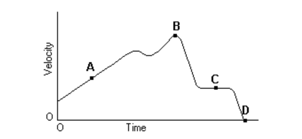
 Above is the graph of the velocity vs. time of a duck flying due south for the winter. At what point might the duck begin reversing directions?
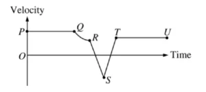 The graph above shows velocity as a function of time for an object moving along a straight line. For which of the following sections of the graph is the acceleration constant and nonzero?
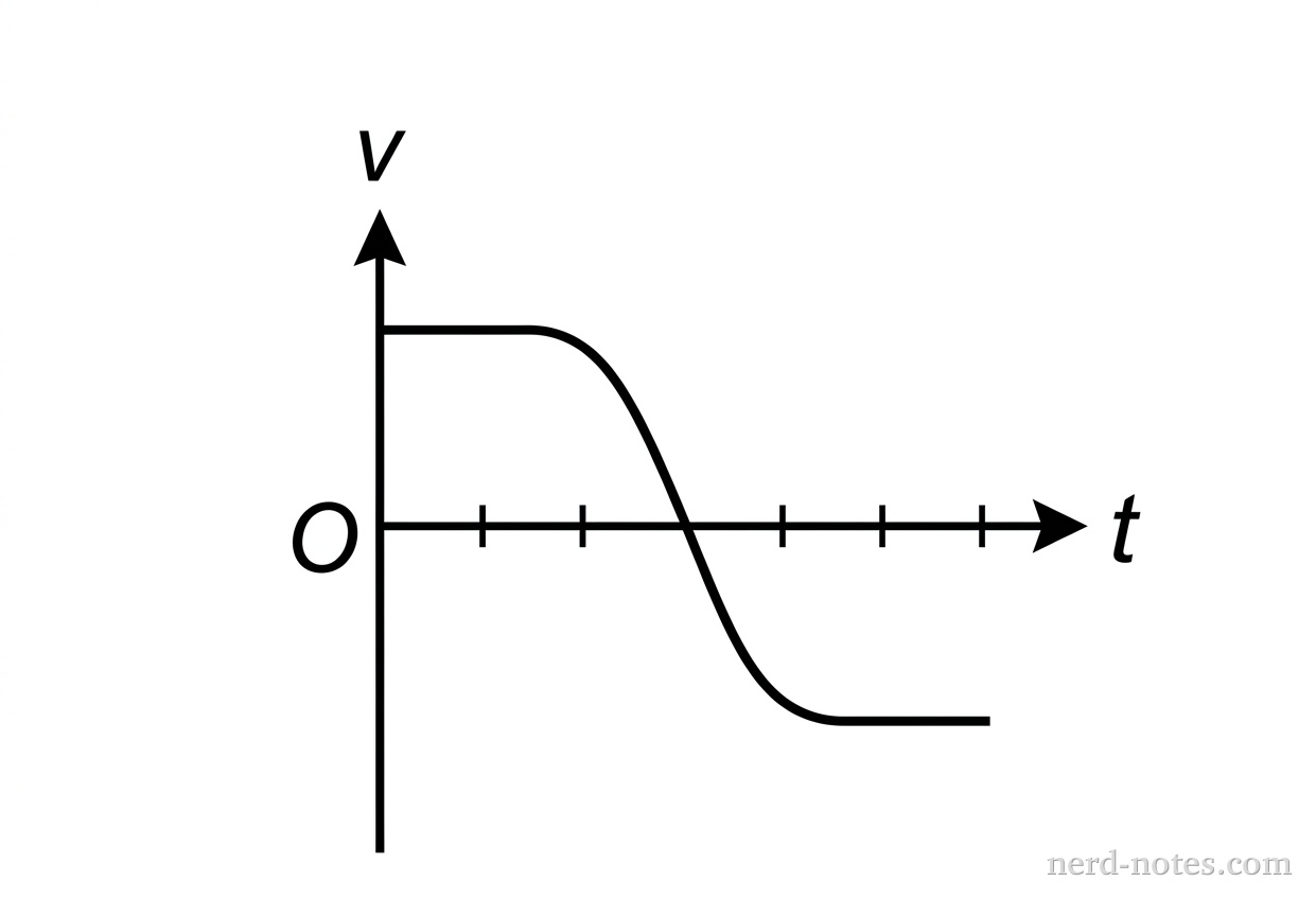
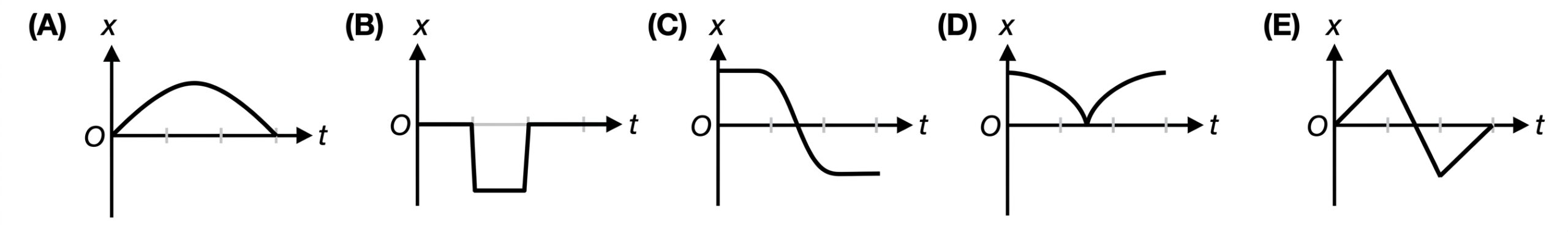
The graph above shows velocity \( v \) versus time \( t \) for an object in linear motion. Which of the following is a possible graph of position (\( x \)) versus time (\( t \)) for this object?
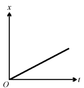
The displacement \( x \) of an object moving in one dimension is shown above as a function of time \( t \). The acceleration of this object must be


