| Step | Derivation/Formula | Reasoning |
|---|---|---|
| 1 | [katex]\text{slope} = \frac{x}{t}[/katex] | The slope of the position vs. time graph represents the velocity of the particle. |
| 2 | [katex]v = 0 \, \text{m/s} \Rightarrow \frac{x}{t} = 0[/katex] | The speed of the particle is [katex]0 \, \text{m/s}[/katex] where the slope of the graph is zero (where the graph becomes flat). |
| 3 | The slope is 0 at [katex] t = 3 \, \text{s} [/katex] | By examining the graph, we notice that the graph is flat at [katex] t = 3 \, \text{s}[/katex], indicating that the velocity is zero. |
A Major Upgrade To Phy Is Coming Soon — Stay Tuned
We'll help clarify entire units in one hour or less — guaranteed.
Which car controls directly allow the driver to cause acceleration?
A driver is driving at \( 40 \, \text{m/s} \) when the light turns red in front of her. It takes the driver \( 0.9 \, \text{s} \) to react and hit the brakes. After this, the car slows with an acceleration of \( 3.5 \, \text{m/s}^2 \). What is the total distance traveled by the car?
A 135.0 N force is applied to a 30.0 kg box at 42 degree angle to the horizontal. If the force of friction is 85.0, what is the net force and acceleration? If the object starts from rest, how far has it traveled in 3.3 sec?
Can an object have a non-zero distance and zero average speed?
Which pair of graphs represents the same 1-dimensional motion?
A student walks \( 3 \) \( \text{m} \) east, then \( 4 \) \( \text{m} \) west in \( 7 \) \( \text{s} \). What is their displacement and average velocity?
A cart begins to move from rest on a horizontal track. Which of the following correctly indicates the magnitude of the average velocity of the cart during the interval shown and provides a valid explanation?
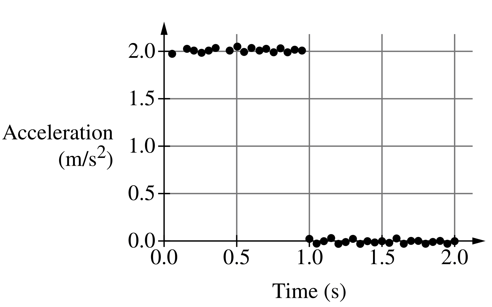
Hint: when solving this, its consider that the area of the acceleration vs time graph tells you the change in velocity.
A body starting from rest moves along a straight line under the action of a constant force. After traveling a distance \( d \) the speed of the body is \( v \). The speed of the body when it has travelled a distance \( \dfrac{d}{2} \) from its initial position is
A rock is dropped from the top of a tall tower. Half a second later another rock, twice as massive as the first, is dropped. Ignoring air resistance and using ONLY simple kinematics (DO NOT use energy to explain this). Explain it like you would to a 5th grader and select the correct choice:
Mary and Sally are in a foot race. When Mary is \( 22 \) \( \text{m} \) from the finish line, she has a speed of \( 4.0 \) \( \text{m/s} \) and is \( 5.0 \) \( \text{m} \) behind Sally, who has a speed of \( 5.0 \) \( \text{m/s} \). Sally thinks she has an easy win and, during the remaining portion of the race, decelerates at a constant rate of \( 0.40 \) \( \text{m/s}^2 \) until she reaches the finish line. What constant acceleration must Mary maintain during the remaining portion of the race if she wishes to cross the finish line side-by-side with Sally?
By continuing you (1) agree to our Terms of Use and Terms of Sale and (2) consent to sharing your IP and browser information used by this site’s security protocols as outlined in our Privacy Policy.
| Kinematics | Forces |
|---|---|
| \(\Delta x = v_i t + \frac{1}{2} at^2\) | \(F = ma\) |
| \(v = v_i + at\) | \(F_g = \frac{G m_1 m_2}{r^2}\) |
| \(v^2 = v_i^2 + 2a \Delta x\) | \(f = \mu N\) |
| \(\Delta x = \frac{v_i + v}{2} t\) | \(F_s =-kx\) |
| \(v^2 = v_f^2 \,-\, 2a \Delta x\) |
| Circular Motion | Energy |
|---|---|
| \(F_c = \frac{mv^2}{r}\) | \(KE = \frac{1}{2} mv^2\) |
| \(a_c = \frac{v^2}{r}\) | \(PE = mgh\) |
| \(T = 2\pi \sqrt{\frac{r}{g}}\) | \(KE_i + PE_i = KE_f + PE_f\) |
| \(W = Fd \cos\theta\) |
| Momentum | Torque and Rotations |
|---|---|
| \(p = mv\) | \(\tau = r \cdot F \cdot \sin(\theta)\) |
| \(J = \Delta p\) | \(I = \sum mr^2\) |
| \(p_i = p_f\) | \(L = I \cdot \omega\) |
| Simple Harmonic Motion | Fluids |
|---|---|
| \(F = -kx\) | \(P = \frac{F}{A}\) |
| \(T = 2\pi \sqrt{\frac{l}{g}}\) | \(P_{\text{total}} = P_{\text{atm}} + \rho gh\) |
| \(T = 2\pi \sqrt{\frac{m}{k}}\) | \(Q = Av\) |
| \(x(t) = A \cos(\omega t + \phi)\) | \(F_b = \rho V g\) |
| \(a = -\omega^2 x\) | \(A_1v_1 = A_2v_2\) |
| Constant | Description |
|---|---|
| [katex]g[/katex] | Acceleration due to gravity, typically [katex]9.8 , \text{m/s}^2[/katex] on Earth’s surface |
| [katex]G[/katex] | Universal Gravitational Constant, [katex]6.674 \times 10^{-11} , \text{N} \cdot \text{m}^2/\text{kg}^2[/katex] |
| [katex]\mu_k[/katex] and [katex]\mu_s[/katex] | Coefficients of kinetic ([katex]\mu_k[/katex]) and static ([katex]\mu_s[/katex]) friction, dimensionless. Static friction ([katex]\mu_s[/katex]) is usually greater than kinetic friction ([katex]\mu_k[/katex]) as it resists the start of motion. |
| [katex]k[/katex] | Spring constant, in [katex]\text{N/m}[/katex] |
| [katex] M_E = 5.972 \times 10^{24} , \text{kg} [/katex] | Mass of the Earth |
| [katex] M_M = 7.348 \times 10^{22} , \text{kg} [/katex] | Mass of the Moon |
| [katex] M_M = 1.989 \times 10^{30} , \text{kg} [/katex] | Mass of the Sun |
| Variable | SI Unit |
|---|---|
| [katex]s[/katex] (Displacement) | [katex]\text{meters (m)}[/katex] |
| [katex]v[/katex] (Velocity) | [katex]\text{meters per second (m/s)}[/katex] |
| [katex]a[/katex] (Acceleration) | [katex]\text{meters per second squared (m/s}^2\text{)}[/katex] |
| [katex]t[/katex] (Time) | [katex]\text{seconds (s)}[/katex] |
| [katex]m[/katex] (Mass) | [katex]\text{kilograms (kg)}[/katex] |
| Variable | Derived SI Unit |
|---|---|
| [katex]F[/katex] (Force) | [katex]\text{newtons (N)}[/katex] |
| [katex]E[/katex], [katex]PE[/katex], [katex]KE[/katex] (Energy, Potential Energy, Kinetic Energy) | [katex]\text{joules (J)}[/katex] |
| [katex]P[/katex] (Power) | [katex]\text{watts (W)}[/katex] |
| [katex]p[/katex] (Momentum) | [katex]\text{kilogram meters per second (kgm/s)}[/katex] |
| [katex]\omega[/katex] (Angular Velocity) | [katex]\text{radians per second (rad/s)}[/katex] |
| [katex]\tau[/katex] (Torque) | [katex]\text{newton meters (Nm)}[/katex] |
| [katex]I[/katex] (Moment of Inertia) | [katex]\text{kilogram meter squared (kgm}^2\text{)}[/katex] |
| [katex]f[/katex] (Frequency) | [katex]\text{hertz (Hz)}[/katex] |
Metric Prefixes
Example of using unit analysis: Convert 5 kilometers to millimeters.
Start with the given measurement: [katex]\text{5 km}[/katex]
Use the conversion factors for kilometers to meters and meters to millimeters: [katex]\text{5 km} \times \frac{10^3 \, \text{m}}{1 \, \text{km}} \times \frac{10^3 \, \text{mm}}{1 \, \text{m}}[/katex]
Perform the multiplication: [katex]\text{5 km} \times \frac{10^3 \, \text{m}}{1 \, \text{km}} \times \frac{10^3 \, \text{mm}}{1 \, \text{m}} = 5 \times 10^3 \times 10^3 \, \text{mm}[/katex]
Simplify to get the final answer: [katex]\boxed{5 \times 10^6 \, \text{mm}}[/katex]
Prefix | Symbol | Power of Ten | Equivalent |
|---|---|---|---|
Pico- | p | [katex]10^{-12}[/katex] | 0.000000000001 |
Nano- | n | [katex]10^{-9}[/katex] | 0.000000001 |
Micro- | µ | [katex]10^{-6}[/katex] | 0.000001 |
Milli- | m | [katex]10^{-3}[/katex] | 0.001 |
Centi- | c | [katex]10^{-2}[/katex] | 0.01 |
Deci- | d | [katex]10^{-1}[/katex] | 0.1 |
(Base unit) | – | [katex]10^{0}[/katex] | 1 |
Deca- or Deka- | da | [katex]10^{1}[/katex] | 10 |
Hecto- | h | [katex]10^{2}[/katex] | 100 |
Kilo- | k | [katex]10^{3}[/katex] | 1,000 |
Mega- | M | [katex]10^{6}[/katex] | 1,000,000 |
Giga- | G | [katex]10^{9}[/katex] | 1,000,000,000 |
Tera- | T | [katex]10^{12}[/katex] | 1,000,000,000,000 |
One price to unlock most advanced version of Phy across all our tools.
per month
Billed Monthly. Cancel Anytime.
We crafted THE Ultimate A.P Physics 1 Program so you can learn faster and score higher.
Try our free calculator to see what you need to get a 5 on the 2026 AP Physics 1 exam.
A quick explanation
Credits are used to grade your FRQs and GQs. Pro users get unlimited credits.
Submitting counts as 1 attempt.
Viewing answers or explanations count as a failed attempts.
Phy gives partial credit if needed
MCQs and GQs are are 1 point each. FRQs will state points for each part.
Phy customizes problem explanations based on what you struggle with. Just hit the explanation button to see.
Understand you mistakes quicker.

Phy automatically provides feedback so you can improve your responses.
10 Free Credits To Get You Started

By continuing you agree to nerd-notes.com Terms of Service, Privacy Policy, and our usage of user data.
Feeling uneasy about your next physics test? We'll boost your grade in 3 lessons or less—guaranteed

NEW! PHY AI accurately solves all questions
🔥 Get up to 30% off Elite Physics Tutoring
🧠 NEW! Learn Physics From Scratch Self Paced Course
🎯 Need exam style practice questions?
