
A \( 0.20 \) \( \text{kg} \) object moves along a straight line. The net force acting on the object varies with the object’s displacement as shown in the graph above. The object starts from rest at displacement \( x = 0 \) and time \( t = 0 \) and is displaced a distance of \( 20 \) \( \text{m} \). Determine each of the following.
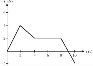
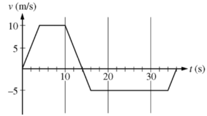
The figure shows the velocity-versus-time graph for a basketball player traveling up and down the court in a straight-line path. Find the displacement of the player…
An object’s velocity \(v\) as a function of time \(t\) is given in the graph. Which of the following statements is true about the motion of the object?
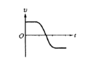
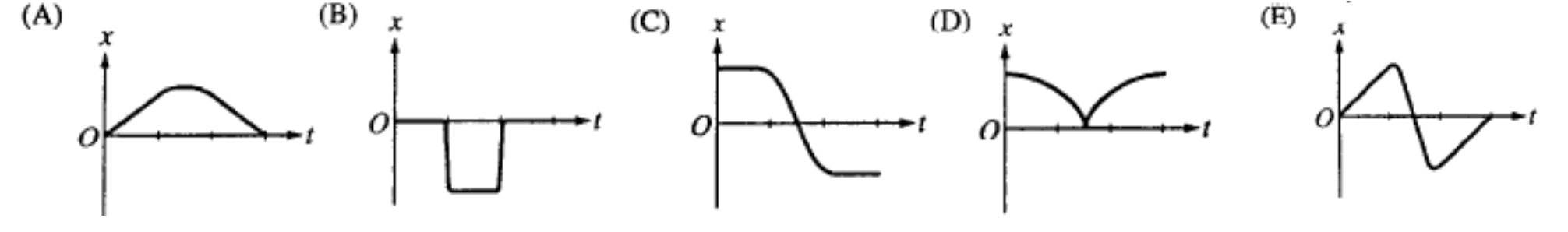
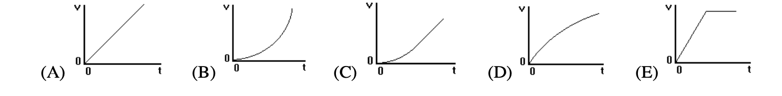
The graph above shows velocity \( v \) versus time \( t \) for an object in linear motion. Which of the following is a possible graph of position (\( x \)) versus time (\( t \)) for this object?
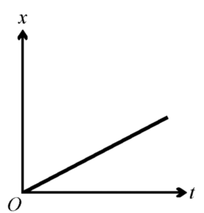
The displacement \( x \) of an object moving in one dimension is shown above as a function of time \( t \). The acceleration of this object must be
A large beach ball is dropped from the ceiling of a school gymnasium to the floor about 10 meters below. Which of the following graphs would best represent its velocity as a function of time? (do not neglect air resistance)
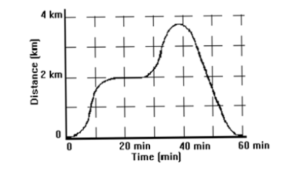
Above is a graph of the \(distance\) vs. time for car moving along a road. According the graph, at which of the following times would the automobile have been accelerating positively?
 The displacement \(x\) of an object moving in one dimension is shown above as a function of time \(t\). The velocity of this object must be


