

Unit 1 Breakdown
You are on Lesson 3 of 5
- Unit 1.1 | Understanding vectors and the Standard Units used in Physics
- Unit 1.2 | The Kinematic (motion) variables: Displacement, Velocity, and Acceleration
- Unit 1.3 | Graphing motion[Current Lesson]
- Unit 1.4 | Using Kinematic Equations in 1 Dimension
- Unit 1.5 | Projectile Motion: Using Kinematic Equations in 2 Dimensions
In this lesson you will learn:
- General graphing principles
- Displacement-time graphs
- Velocity-time graphs
- Acceleration-time graphs
- Converting one graph from another
- Creating graphs from real-world scenarios
Introduction
Motion graphs, as well as other graphs, will show up throughout out tests.
The goal of this lesson is not only to learn about kinematic graphs, but also learn to logically understand all types of graphs. This lesson will save you from tons of future headaches!
The 3 Motion Graphs
Here are the three motion graphs (aka kinematic graphs) we will cover in this lesson:
- position-time
- velocity-time
- acceleration-time
Remember the following — for ANY line-graph there are 3 actions we can take:
- Action 1: Find a point along the line
- Action 2: Find the slope of the line
- Action 3: Find the area between the line and the x-axis (a.k.a the area under the curve)
For each of the the 3 graphs we will explain what each action represents.
For example, the action of finding the slope on a position-time graph, represents velocity.
While you can apply these actions to every graph, the number you get from each action might not represent anything meaningful.
For example, the area under the curve of a position time graph does not tell us anything.
Graph 1: Position-time
On a position-time graph, we can use two actions to get two meaningful results.
Here’s what each action means for position-time graphs:
- Action 1: finding a point on the line = an object’s instantaneous position
- Action 2: finding the slope of the line = an object’s velocity
- Action 3: area under curve: means NOTHING!
Let’s cover each one.
Instantaneous Position
The instantaneous position is a point on the position-time graph, at a particular second. It represent the position at that instant.
For example, look at the graph below and place your finger anywhere along the line.
The point where your finger lies is the position of the object at THAT instant.
Velocity
The slope, of the position-time graph line, tells us the object’s velocity.
Why?
Using the same graph above let’s find the slope, but in terms of the units.
Slope = rise divided by run = m ÷ s. The units of the slope is m per second, which is velocity (how fast something is moving)
So…the slope of the line gives the velocity: [katex] v = \frac{\Delta x}{\Delta t} [/katex].
Try this: Using the graph above find the object’s velocity.
Answer: the velocity is simply the slope of the line. The slope is rise/run = 15 m ÷ 5 s = 3 m/s.
5 position-time graphs
Here are 5 common position-time graphs and what each action item means.
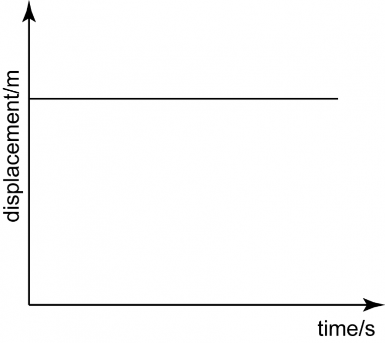
Horizontal line = 0 slope = 0 velocity
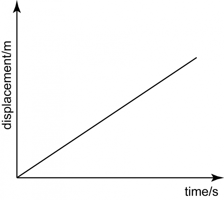
Linear upwards sloping line = constant positive slope = constant positive velocity
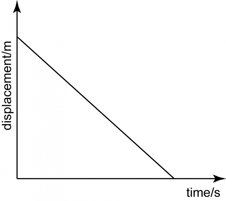
Linear downwards sloping line = constant negative slope = constant negative velocity

Non-constant upwards sloping curve. The slope is increasing = increasing positive velocity
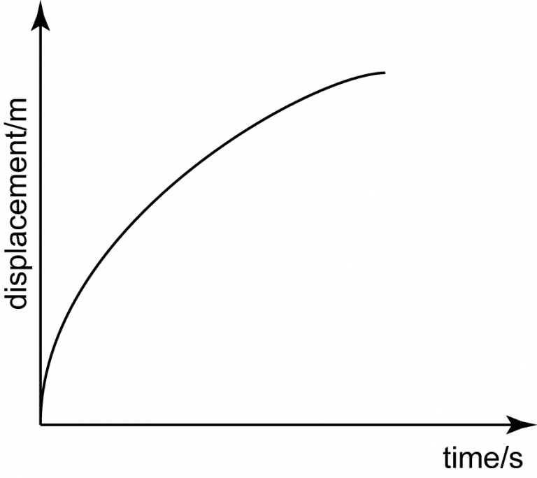
Non-constant upwards sloping curve. The slope is decreasing = decreasing positive velocity
Graph 2: Velocity-time
On a position-time graph, we can use three actions to get three meaningful results:
- Action 1: finding a point on the line = an object’s instantaneous velocity
- Action 2: finding the slope of the line = an object’s acceleration
- Action 3: finding the area under the line = an object’s total displacement
Let’s cover each one.
Instantaneous speed
The instantaneous speed is a point on the graph, at a particular second. It represent the speed at that instant.
For example, on the velocity-time graph below, place your finger anywhere along the line.
Where your finger lays is the velocity at that instant.

Acceleration
To find acceleration, we find the slope of the line.
Why?
Slope is rise divided by run. Look at the units of “rise.” It’s ‘m/s’. Now look at the units of “run” it’s ‘s’.
So the slope in terms of units = m/s ÷ s, which is the same thing as m/s2 (the unit for acceleration).
In other words: [katex] slope = \frac{\Delta v}{\Delta t} = acceleration[/katex]
Try this: Using the graph above find the velocity from 2 to 5 seconds.
Answer
From 2 to 5 seconds the line is completely flat, thus the slope is 0. Remember that the slope on a position-time graph represent velocity. So: 0 slope = 0 velocity.
Displacement
Finally, we can find the displacement, by calculating the area bound by the line and the x-axis.
Why? Once again, let’s look at the units.
To find area, we must multiply the numbers along the x and y axis. In terms of units this will be ‘s’ x ‘m/s’. We can simplify and cancel out ‘s’ and our final unit is just ‘m’. Meters (m) is the unit for displacement.
So multiplying velocity (on the y axis) and time (on the x-axis) will tell us the displacement (∆x).
In other words, area under curve:
[katex] \Delta v \times \Delta t = \Delta x [/katex]
Try this: using the graph above, find the displacement in the first two seconds.
Answer
In the first 2 seconds the line makes a triangle shape with the x axis. To find displacement, we must find the area of the triangle: [katex] \frac{1}{2}\time b \time h = \frac{1}{2}\time 2 \times 30 = 30 \, m/s[/katex].
5 Velocity-time graphs
Below are 5 common velocity-time graphs you will come across.
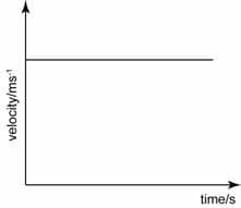
Horizontal line = 0 slope = 0 velocity
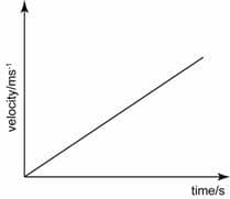
Linear upwards sloping line = constant positive slope = constant positive velocity
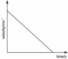
Linear downwards sloping line = constant negative slope = constant negative velocity
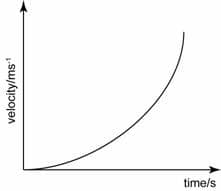
Non-constant upwards sloping curve. The slope is increasing = increasing positive velocity
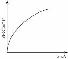
Non-constant upwards sloping curve. The slope is decreasing = decreasing positive velocity
Graph 3: Acceleration-time
This is the final graph!
On a acceleration-time graph, we can use two actions to get two meaningful results:
- Action 1: finding a point on the line = an object’s instantaneous acceleration
- Action 2: slope = NOTHING!
- Action 3: finding the area under the line = an object’s total change in velocity
Let’s cover each one.
Instantaneous Acceleration
The instantaneous acceleration is a point on the graph, at a particular second. It represent the acceleration at that instant.
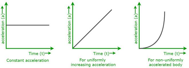
Here are three types of instantaneous accelerations, shown on the green graphs below.
- Constant acceleration – A straight, horizontal line indicates constant acceleration (the only you will use your first Physics course)
- Increasing acceleration – A uniform upwards (positive) sloping line
- Decreasing acceleration – A uniform downwards (negative) sloping line
Total Change in Velocity
As in the previous graphs lets use units to determine what the area under the curve means.
Finding area means we multiply acceleration (the y-axis), by the time (x-axis).
So in terms of units that is m/s2 x s. This simplifies down to m/s which is unit of velocity (v)
In other words, area under curve
[katex] \Delta a \times \Delta t = v [/katex]
Cheat Sheet
| Graph | Point on Graph | Slope of Graph | Area Under Graph |
|---|---|---|---|
| Displacement-time | instantaneous position | velocity | nothing meaningful |
| Velocity-time | instantaneous velocity | acceleration | displacement |
| Acceleration-time | instantaneous acceleration | nothing meaningful | velocity |
Other Graphs in Physics
As you cover more chapters, you will come across more graphs, like force-time, energy-distance graphs, etc.
Now that you understand the basics of motion graphs, it’s important to use our logic skills to extend this to all other graphs.
Two important things you must remember is taking the slope of the line and the area under any graph. You can figure out what these quantities mean by looking at formulas of units.
For example, lets suppose we are working with a Force-acceleration graph. What would the slope of the graph represent?
The slope would be Force divided by acceleration, which is equal to mass, as you’ll learn in unit 2.
PQ – Motion Graphs
Before continuing complete the worksheet below, to test your understanding so far. Remember to review all missed questions.
LRN Making and Converting Graphs
We’ve spent a lot of time going over graphs and what they mean.
Now we will take our new knowledge to do the following:
- Convert from one graph to another. Example: make a velocity-time graph from the given displacement-time graph
- Turn a situation into a graph. Example: make a velocity graph for a ball being thrown upwards.
This can be complicated to explain in writing, so we recommend watching the detailed video below.

Lesson 1.4 Preview
Now that we’re done with kinematic (motion) graphs, we can move on to solving motion questions. In the next lesson we will use kinematic equations to solve real-world problems. This is a fun and easy lesson for many students!
